31  Gaussian mixture

library(dplyr)
# required for figures  
library(ggplot2)
library(gridExtra)
# required for render latex 
library(backports)
library(latex2exp)
# required for render tables
library(knitr)
library(kableExtra)
library(solarr)
# Random seed 
set.seed(1)

Let’s consider a linear combination of a Bernoulli and two normal random variables, all assumed to be independent, i.e. $$\begin{array}{}\text{(31.1)}& X_t\sim B_t\cdot X_{1,t}+(1-B_t)\cdot X_{0,t}\text{,}\end{array}$$ where $B$ is a Bernoulli random variable $$B_t\sim \text{Bernoulli}(p)\text{,}$$ and for the $i$-th component $$X_{i,t}={\mu }_1+{\sigma }_1{Z}_{i,t}$$ where $Z_{i,t}$ is standard Normal random variable. In compact form a Gaussian Mixture with two components is denoted as $X_t\sim GM({\mu }_1,{\mu }_0,{\sigma }_1^2,{\sigma }_0^2,p)$.

(a) Simulated mixture sample.

(b) Simulated (black) and true (red) density.

(c) Simulated (black) and true (red) distribution.

Figure 31.1: Gaussian Mixture simulation and density function with true parameters ${\mu }_1=-2$, ${\mu }_2=2$, ${\sigma }_1=1$, ${\sigma }_2=1$ and $p=0.5$.

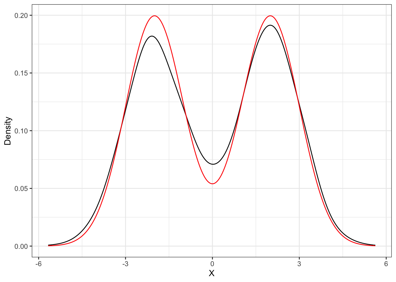
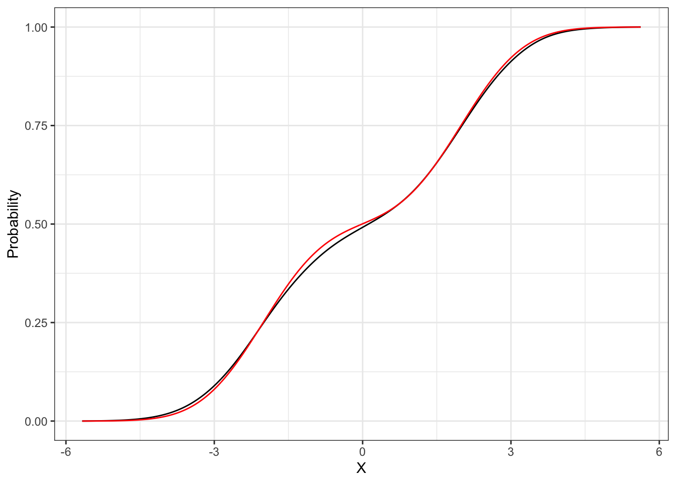
31.1 Distribution and density

Proposition 31.1 The distribution function of a Gaussian mixture random variable is a weighted sum between the distributions of the components, i.e.: $$\begin{array}{}\text{(31.2)}& F_X(x)=p\cdot F_{X_1}(x)+(1-p)F_{X_0}(x)\text{,}\end{array}$$ Taking the derivative, it can be easily shown that the density function reads: $$\begin{array}{}\text{(31.3)}& f_X(x)=p\cdot f_{X_1}(x)+(1-p)f_{X_0}(x)\text{.}\end{array}$$ In general $$\begin{array}{}\text{(31.4)}& f_X(x)=\frac{p}{{\sigma }_1}\cdot \varphi \left(\frac{x-{\mu }_1}{{\sigma }_1}\right)+\frac{1-p}{{\sigma }_0}\cdot \varphi \left(\frac{x-{\mu }_0}{{\sigma }_0}\right)\text{,}\end{array}$$ where $\mathrm{\Phi }$ is the cumulative distribution function and $\varphi$ is the density function of a standard normal random variable. An implementation of the density and distribution of a Gaussian Mixture is contained in the R package extraDistr, i.e. dmixnorm for the density and pmixnorm for the distribution.

Proof: Proposition 31.1

Proof. From the formal definition of distribution function of a random variable $X$ $$F_X(y)=\mathbb{P}(X\le y)=\mathbb{E}\{{\mathbb{1}}_{X\le x}\}\text{,}$$ where if $X$ is a Gaussian Mixture with two components we can express it as conditional expectation with respect to $B$, i.e.  $$\begin{array}{rl}{F}_X(y)& =\mathbb{E}\{{\mathbb{1}}_{X\le x}|B\}=\\ & =\mathbb{E}\{{\mathbb{1}}_{X\le x}|B=0\}\mathbb{P}(B=0)+\mathbb{E}\{{\mathbb{1}}_{X\le x}\mid B=1\}\mathbb{P}(B=1)=\\ & =p\cdot \mathbb{P}(X_1\le x)+(1-p)\cdot \mathbb{P}(X_0\le x)\end{array}$$ Hence, standardizing the Normal random variable one obtain $$F_X(x)=p\cdot \mathrm{\Phi }\left(\frac{x-{\mu }_1}{{\sigma }_1}\right)+(1-p)\cdot \mathrm{\Phi }\left(\frac{x-{\mu }_0}{{\sigma }_0}\right)\text{,}$$ where $\mathrm{\Phi }$ denotes the distribution function of a standard normal. Knowing that $f_X(x)=\frac{d{F}_X(x)}{dx}$ and that ${\varphi }_X(x)=\frac{d\mathrm{\Phi }(x)}{dx}$, where $\varphi$ is the density function of a standard normal we obtain the result, i.e. $$f_X(x)=\frac{p}{{\sigma }_1}\cdot \varphi \left(\frac{x-{\mu }_1}{{\sigma }_1}\right)+\frac{1-p}{{\sigma }_0}\cdot \varphi \left(\frac{x-{\mu }_0}{{\sigma }_0}\right)\text{.}$$

31.2 Moment generating function

Proposition 31.2 The moment generating function of a Gaussian mixture random variable (Equation 31.1) in $t$ reads: $$M_X(u)=p\cdot M_{X_1}(u)+(1-p)\cdot M_{X_0}(u)\text{.}$$ where for a general $i\in \{0,1\}$, $M_{X_i}(u)$ is the moment generating function of a Gaussian random variable with moments ${\mu }_i$, ${\sigma }_i^2$, i.e. $$\begin{array}{rl}{M}_{X_i}(u)& =\exp \{{\mu }_{i}u+\frac{u^2{\sigma }_i^2}{2}\}\end{array}$$

Proof: Proposition 31.2

Proof. Applying the definition of moment generating function and the property of linearity of the expectation on a Gaussian mixture (Equation 31.1), one obtain: $$\begin{array}{rl}{M}_X(u)& =p\cdot \mathbb{E}\{e^{u{Z}_1}\}+(1-p)\cdot \mathbb{E}\{e^{u{Z}_0}\}=\\ & =p\cdot M_{X_1}(u)+(1-p)\cdot M_{X_0}(u)\end{array}$$ Hence, the moment generating function of $X$ is a linear combination of the moment generating functions of the two components.

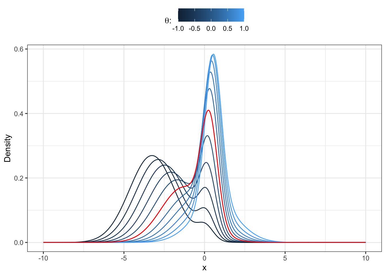
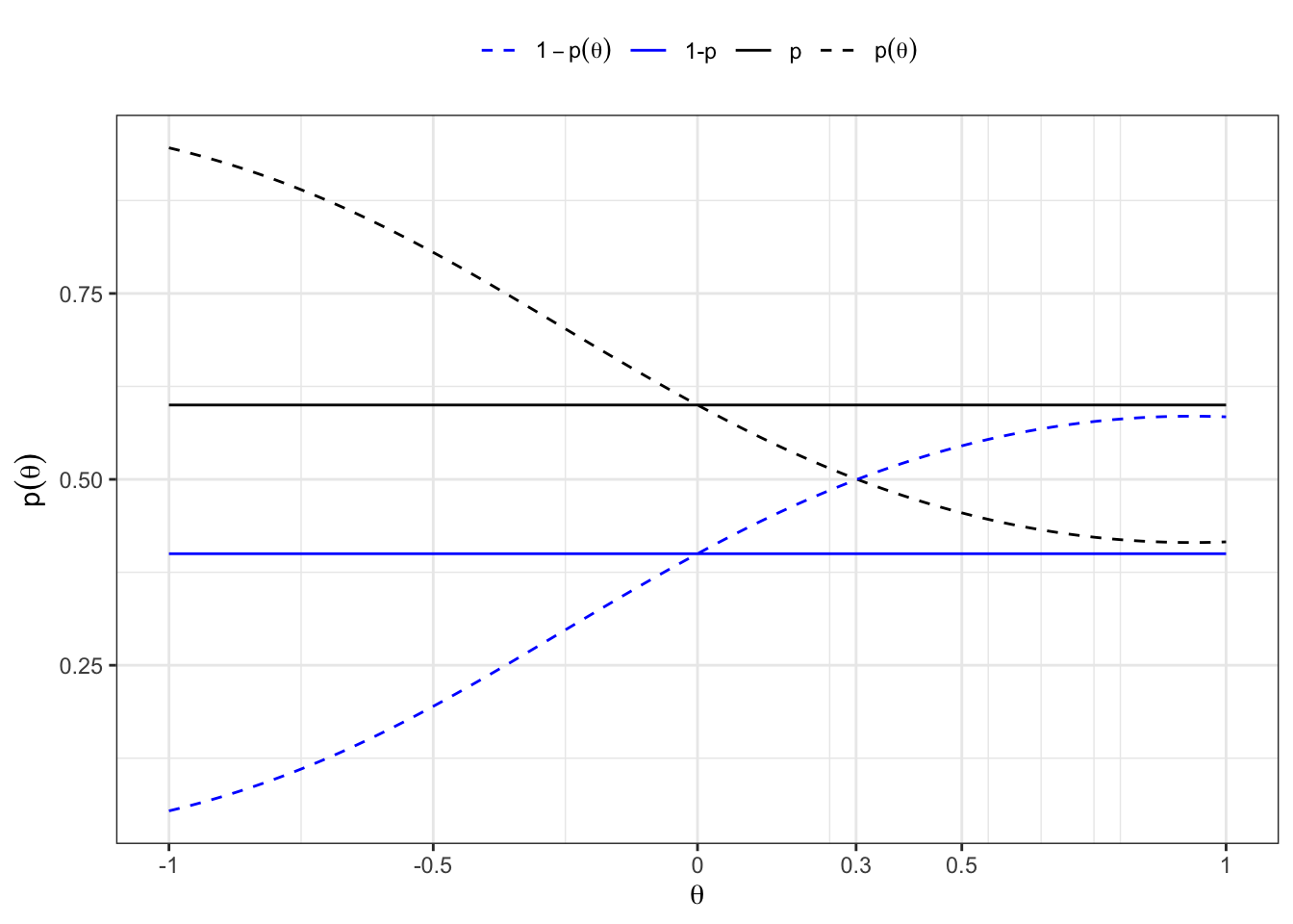
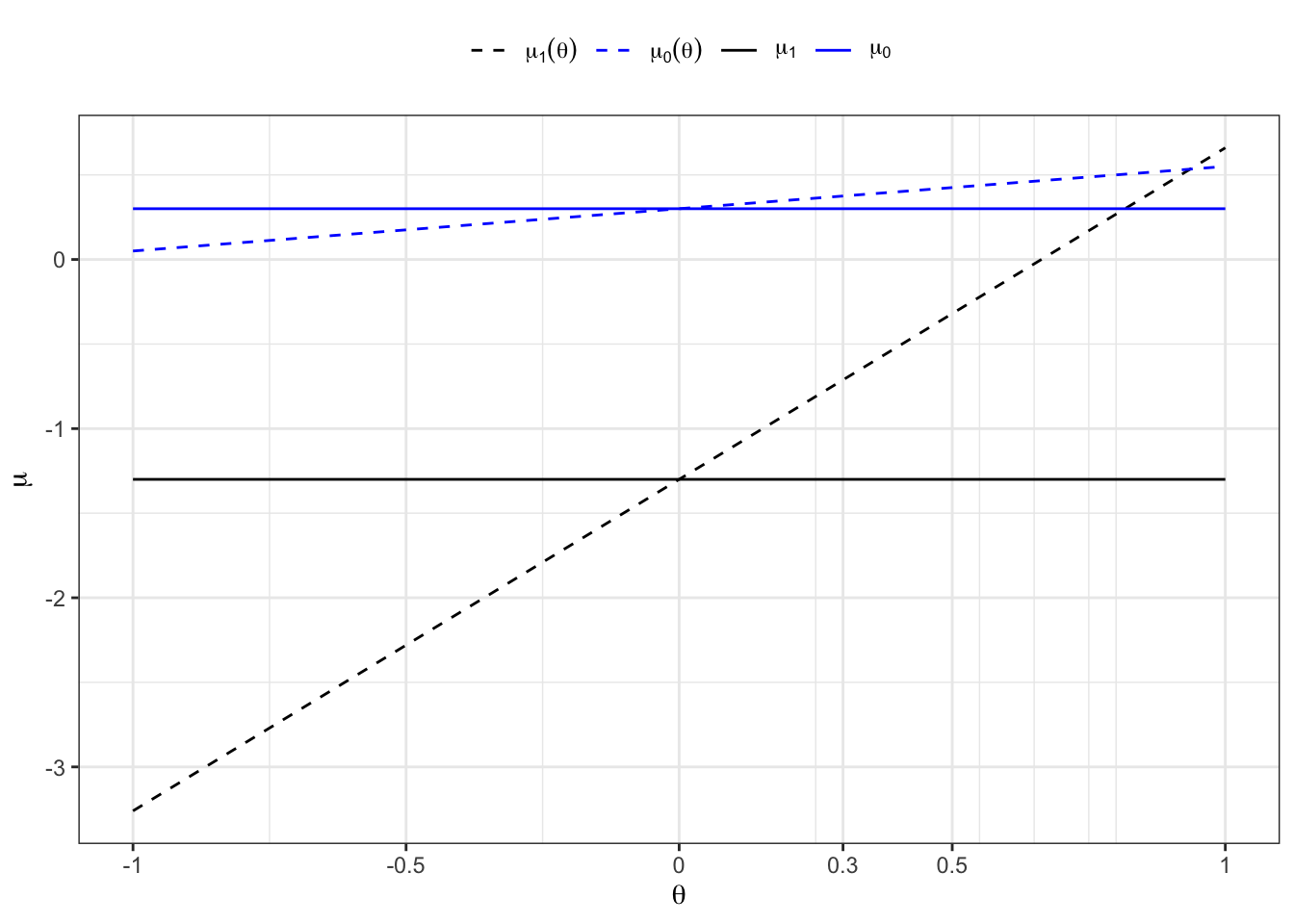
31.3 Esscher transform

Proposition 31.3 The Esscher transform of a Gaussian mixture random variable reads: $${\mathcal{E}}_{\theta }\{f_X\}(x)=p_1(\theta )f_{X_1}(x;\theta )+p_0(\theta )f_{X_0}(x;\theta )\text{,}$$ where for $i\in \{0,1\}$: $$f_X(x;\theta )=\frac{1}{{\sigma }_i}\varphi \left(\frac{x-{\mu }_i-\theta {\sigma }_i^2}{{\sigma }_i}\right)\text{,}$$ and the distorted probabilities are defined as: $$p_1(\theta )=p\cdot \frac{M_{X_1}(\theta )}{M_X(\theta )}\text{,}{p}_0(\theta )=(1-p_1(\theta ))\text{.}$$

Proof: Proposition 31.3

Proof. In general, the Esscher transform of a density function $f_X$ is defined as:
$${\mathcal{E}}_{\theta }\{f_X\}(x)=\frac{e^{\theta x}{f}_X(x)}{M_X(\theta )}=\frac{e^{\theta x}{f}_X(x)}{{\int }_{-\mathrm{\infty }}^{\mathrm{\infty }}{e}^{\theta y}{f}_X(y)dy}\text{.}$$ Let’s focus only on the numerator. Substituting the density function of a Gaussian mixture one obtain: $${\mathcal{E}}_{\theta }\{f_X\}(x)=\frac{e^{\theta X}(p{f}_{Z_1}(x)+(1-p)f_{Z_2}(x))}{M_X(\theta )}\text{.}$$ Let’s consider the $i$-component for $i\in \{0,1\}$ and let’s explicit the density function, i.e. $$e^{\theta x}{f}_{Z_i}(x)=\frac{1}{\sqrt{2\pi }{\sigma }_i^2}\exp \{-\frac{(x-{\mu }_i{)}^2}{2{\sigma }_i^2}+\theta x\}\text{.}$$ Let’s expand the exponent of the exponential term for the $i$-th component, i.e.  $$\begin{array}{rl}\theta x-\frac{(x-\mu {)}^2}{2{\sigma }^2}& =\theta x-\frac{x^2-2\mu x+{\mu }^2}{2{\sigma }^2}=\\ & =-\frac{x^2}{2{\sigma }^2}+(\theta +\frac{\mu }{{\sigma }^2})x-\frac{{\mu }^2}{2{\sigma }^2}\end{array}$$ Let’s denote with $A=\theta +\frac{\mu }{{\sigma }^2}$, then complete the square $$-\frac{x^2}{2{\sigma }^2}+Ax=-\frac{1}{2{\sigma }^2}[x^2-2{\sigma }^{2}Ax+A^2{\sigma }^4]+\frac{A^2{\sigma }^2}{2}=\frac{(x-A{\sigma }^2)}{2{\sigma }^2}+\frac{A^2{\sigma }^2}{2}\text{,}$$ Therefore $$\begin{array}{rl}\theta x-\frac{(x-{\mu }_i{)}^2}{2{\sigma }_i^2}& =\frac{(x-{\mu }_i-\theta {\sigma }^2)}{2{\sigma }_i^2}-\frac{{\mu }_i^2}{2{\sigma }_i^2}+\frac{(\theta {\sigma }_i^2+\mu {)}^2}{2{\sigma }_i^2}=\\ & =\frac{(x-{\mu }_i-\theta {\sigma }_i^2)}{2{\sigma }_i^2}-\frac{{\mu }_i^2}{2{\sigma }_i^2}+\frac{{\theta }^2}{2}+\frac{{\mu }_i^2}{2{\sigma }_i^2}+\theta {\mu }_i=\\ & =\frac{(x-{\mu }_i-\theta {\sigma }_i^2)}{2{\sigma }_i^2}+\frac{{\theta }^2}{2}+\theta {\mu }_i\end{array}$$ Hence, adding and subtracting inside the exponential one obtain $$\begin{array}{rl}{e}^{\theta x}{f}_{Z_i}(x)& =\frac{1}{\sqrt{2\pi }{\sigma }_i}\exp \{-\frac{(x-{\mu }_i{)}^2}{2{\sigma }_i^2}+\theta x-{\mu }_i\theta -\frac{{\theta }^2{\sigma }_i^2}{2}\}\exp \left\{{\mu }_i\theta +\frac{{\theta }^2{\sigma }_i^2}{2}\right\}=\\ & =\frac{1}{\sqrt{2\pi }{\sigma }_i}\exp \{{\mu }_i\theta +\frac{\theta {\sigma }_i^2}{2}\}\exp \{-\frac{(x-{\mu }_i-\theta {\sigma }_i^2{)}^2}{2{\sigma }_i^2}\}=\\ & =M_{Z_i}(\theta )f_{Z_i}(x;\theta )\end{array}$$ Hence, we obtain the result $$f_{Z_i}(x;\theta )=\frac{1}{{\sigma }_i}\varphi \left(\frac{x-{\mu }_i-\theta {\sigma }_i^2}{{\sigma }_i}\right)\text{.}$$ Hence, the Esscher density $${\mathcal{E}}_{\theta }\{f_X\}(x)=\frac{p{M}_{Z_1}(\theta )f_{Z_1}(x;\theta )+(1-p)M_{Z_0}(\theta )f_{Z_i}(x;\theta )}{M_X(\theta )}\text{.}$$ Hence let’s collect the first part and the denominator (mgf of the Gaussian mixture in $\theta$) and define the new probabilities $$p_1(\theta )=\frac{p{M}_{X_1}(\theta )}{M_X(\theta )}\text{,}{p}_0(\theta )=\frac{(1-p)M_{X_0}(\theta )}{M_X(\theta )}\text{.}$$

(a) Esscher densities for different values of $\theta$ in $[-1,1]$ and with $\theta =0$ (red).

(b) Distorted mixture probability for different values of $\theta$ in $[-1,1]$ and with $\theta =0$ (red).

(c) Distorted mixture means for different values of $\theta$ in $[-1,1]$ and with $\theta =0$ (red).

Figure 31.2: Esscher transform of a Gaussian mixture.

31.4 Moments

Proposition 31.4 The expectation of a Gaussian Mixture random variable (Equation 31.1) reads: $$\begin{array}{}\text{(31.5)}& \mathbb{E}\{X\}=p{\mu }_1+(1-p){\mu }_2\text{,}\end{array}$$ and the second moment $$\begin{array}{}\text{(31.6)}& \mathbb{E}\{X^2\}=p({\mu }_1^2+{\sigma }_1^2)+(1-p)({\mu }_2^2+{\sigma }_2^2)\text{.}\end{array}$$ Hence, the variance
$$\begin{array}{}\text{(31.7)}& \mathbb{V}\{X\}=p(1-p)({\mu }_1-{\mu }_2{)}^2+{\sigma }_1^{2}p+{\sigma }_2^2(1-p)\text{.}\end{array}$$

Proof: Proposition 31.4

Proof. Given that $X_1$, $X_0$ and $B$ are independent, the expectation is computed as: $$\begin{array}{rl}\mathbb{E}\{X\}& =\mathbb{E}\{\mathbb{E}\{X\mid B\}\}=\\ & =\mathbb{E}\{X\mid B=1\}\mathbb{P}(B=1)+\mathbb{E}\{X\mid B=0\}\mathbb{P}(B=0)=\\ & =p\mathbb{E}\{X_1\}+(1-p)\mathbb{E}\{X_0\}=\\ & =p{\mu }_1+(1-p){\mu }_2\end{array}$$ The second moment is computed similarly to the first one, i.e.  $$\begin{array}{rl}\mathbb{E}\{X^2\}& =\mathbb{E}\{\mathbb{E}\{X^2\mid B\}\}=\\ & =\mathbb{E}\{X^2\mid B=1\}\mathbb{P}(B=1)+\mathbb{E}\{X^2\mid B=0\}\mathbb{P}(B=0)=\\ & =\mathbb{E}\{B\}\mathbb{E}\{X_1^2\}+\mathbb{E}\{1-B\}\mathbb{E}\{X_0^2\}=\\ & =p\mathbb{E}\{X_1^2\}+(1-p)\mathbb{E}\{X_0^2\}=\\ & =p({\mu }_1^2+{\sigma }_1^2)+(1-p)({\mu }_2^2+{\sigma }_2^2)\end{array}$$ The variance, by definition, is given by: $$\mathbb{V}\{X\}=\mathbb{E}\{X^2\}-\mathbb{E}\{X{\}}^2\text{,}$$ where the first moment squared is $$\begin{array}{}\text{(31.8)}& \begin{array}{rl}\mathbb{E}\{X{\}}^2& ={(p{\mu }_1+(1-p){\mu }_2)}^2=\\ & =p^2{\mu }_1^2+(1-p{)}^2{\mu }_2^2+2p(1-p){\mu }_1{\mu }_2\end{array}\end{array}$$ Hence the variance, $$\begin{array}{rl}\mathbb{V}\{X\}& =p({\mu }_1^2+{\sigma }_1^2)+(1-p)({\mu }_2^2+{\sigma }_2^2)-p^2{\mu }_1^2-(1-p{)}^2{\mu }_2^2-2p(1-p){\mu }_1{\mu }_2=\\ & =p{\mu }_1^2+p{\sigma }_1^2+{\mu }_2^2+{\sigma }_2^2-p{\mu }_2^2-p{\sigma }_2^2-p^2{\mu }_1^2-(1-p{)}^2{\mu }_2^2-2p(1-p){\mu }_1{\mu }_2=\\ & ={\mu }_1^{2}p(1-p)+p{\sigma }_1^2+(1-p){\sigma }_2^2+p(1-p){\mu }_2^2-2p(1-p){\mu }_1{\mu }_2=\\ & =p(1-p)({\mu }_1^2-{\mu }_2^2-2{\mu }_1{\mu }_2)+p{\sigma }_1^2+(1-p){\sigma }_2^2=\\ & =p(1-p)({\mu }_1-{\mu }_2{)}^2+p{\sigma }_1^2+(1-p){\sigma }_2^2\end{array}$$ Equivalently, with the law of total variance: $$\mathbb{V}\{X\}=\mathbb{V}\{\mathbb{E}\{X\mid B\}\}+\mathbb{E}\{\mathbb{V}\{X\mid B\}\}$$ where $$\begin{array}{rl}\mathbb{E}\{\mathbb{V}\{X\mid B\}\}& =\mathbb{E}\{{\sigma }_1^{2}B+{\sigma }_0^2(1-B)\}=\\ & ={\sigma }_1^{2}p+{\sigma }_0^2(1-p)\end{array}$$ Then $$\begin{array}{rl}\mathbb{E}\{X\mid B\}& ={\mu }_{1}B+{\mu }_0(1-B)=\\ & ={\mu }_0+({\mu }_1-{\mu }_0)B\end{array}$$ and therefore $$\begin{array}{rl}\mathbb{V}\{\mathbb{E}\{X\mid B\}\}& =\mathbb{V}\{{\mu }_0+({\mu }_1-{\mu }_0)B\}=\\ & =({\mu }_1-{\mu }_0{)}^2\mathbb{V}\{B\}=\\ & =({\mu }_1-{\mu }_0{)}^{2}p(1-p)\end{array}$$ The total variance: $$\begin{array}{rl}\mathbb{V}\{X\}& =\mathbb{V}\{\mathbb{E}\{X\mid B\}\}+\mathbb{E}\{\mathbb{V}\{X\mid B\}\}=\\ & =({\mu }_1-{\mu }_0{)}^{2}p(1-p)+{\sigma }_1^{2}p+{\sigma }_0^2(1-p)\end{array}$$

31.4.1 Special Cases

Proposition 31.5 If the random variable $X$ (Equation 31.1) is centered in zero, i.e. $$\mathbb{E}\{X\}=p{\mu }_1+(1-p){\mu }_0=0\text{,}$$ then, the following expression holds $$({\mu }_1-{\mu }_0{)}^{2}p(1-p)=p{\mu }_1^2+(1-p){\mu }_0^2$$

Proof: Proposition 31.5

Proof. Let’s show that the following expressions $$\text{LHS}=p(1-p)({\mu }_1-{\mu }_0{)}^2\equiv p{\mu }_1^2+(1-p){\mu }_0^2=\text{RHS}$$ are equivalent under the constraint $$\mathbb{E}\{X\}=p{\mu }_1+(1-p){\mu }_0=0$$ Firstly let’s note that if the mixture is centered the ration between ${\mu }_1$ and ${\mu }_0$ is constant, i.e. $${\mu }_{1}p+{\mu }_0(1-p)=0⟹{\mu }_1=-{\mu }_{0}r$$ where we define the ratio $r$ as: $$r=\frac{(1-p)}{p}$$ Let’s now expand the LHS and substitute the relation between ${\mu }_1$ and ${\mu }_0$: $$\begin{array}{rl}\text{LHS}& =({\mu }_1-{\mu }_0{)}^{2}p(1-p)=\\ & =p(1-p){\mu }_1^2-2p(1-p){\mu }_1{\mu }_0+p(1-p){\mu }_0^2=\\ & =p(1-p)(r^2{\mu }_0^2+2r{\mu }_0^2+{\mu }_0^2)=\\ & =p(1-p){\mu }_0^2(r^2+2r+1)=\\ & =p(1-p){\mu }_0^2(r+1{)}^2\end{array}$$ Then, we note that $$(r+1)=(\frac{1-p}{p}+1)=\frac{1-p+p}{p}=\frac{1}{p}⟹\text{LHS}={\mu }_0^2\frac{1-p}{p}$$ Now, let’s consider the RHS $$\begin{array}{rl}\text{RHS}& =p{\mu }_1^2+(1-p){\mu }_0^2=\\ & =p{r}^2{\mu }_0^2+(1-p){\mu }_0^2=\\ & ={\mu }_0^2(p{r}^2+1-p)=\\ & ={\mu }_0^2\frac{1-p}{p}\end{array}$$ since $$\begin{array}{rl}(p{r}^2+1-p)& =(p\frac{(1-p{)}^2}{p^2}+1-p)=\\ & =\left(\frac{(1-p{)}^2+p(1-p)}{p}\right)=\\ & =(1-p)\left(\frac{1-p+p}{p}\right)=\\ & =\frac{1-p}{p}\end{array}$$ Hence, the RHS and LHS are equal.

31.4.2 Central moments

Proposition 31.6 The second central moment of a Gaussian mixture reads: $${\kappa }_2\{X\}=({\delta }_1^2+{\sigma }_1^2)p+({\delta }_0^2+{\sigma }_0^2)(1-p)=\mathbb{V}\{X\}$$ where for $i\in \{0,1\}$, ${\delta }_i={\mu }_i-\mathbb{E}\{X\}$.

Proof: Proposition 31.6

Proof. Developing the squares: $$\begin{array}{rl}& {\delta }_1^2=({\mu }_1^2+\mathbb{E}\{X{\}}^2-2{\mu }_1\mathbb{E}\{X\})\\ & {\delta }_0^2=({\mu }_0^2+\mathbb{E}\{X{\}}^2-2{\mu }_0\mathbb{E}\{X\})\end{array}$$ and summing $$\begin{array}{rl}& {\delta }_1^{2}p+{\delta }_0^2(1-p)=({\mu }_1^{2}p+{\mu }_0^2(1-p))+\mathbb{E}\{X{\}}^2-2({\mu }_{1}p+{\mu }_0(1-p))\mathbb{E}\{X\}=\\ & =({\mu }_1^{2}p+{\mu }_0^2(1-p))-\mathbb{E}\{X{\}}^2\end{array}$$ Thus, substituting the result in the initial expression one obtain the result.

31.5 Estimation

31.5.1 Maximum likelihood

Minimizing the negative log-likelihood gives an estimate of the parameters, i.e. $$\underset{{\mu }_1,{\mu }_2,{\sigma }_1,{\sigma }_2,p}{\text{argmin}}\{\sum _{i=1}^t\log (f_X(x_i))\}\text{,}$$ or equivalently maximizing the negative log-likelihood, i.e.  $$\underset{{\mu }_1,{\mu }_2,{\sigma }_1,{\sigma }_2,p}{\text{argmax}}\{-\sum _{i=1}^t\log (f_X(x_i))\}\text{.}$$

Example: ML-estimate

# Initialize parameters 
init_params <- par*runif(5, 0.3, 1.1)
# Log-likelihood loss function
loss <- function(params, x){
  # Parameters
  mu1 = params[1]
  mu2 = params[2]
  sd1 = params[3]
  sd2 = params[4]
  p = params[5]
  # Ensure that probability is in (0,1)
  if(p > 0.99 | p < 0.01 | sd1 < 0 | sd2 < 0){ s
    return(NA_integer_)
  }
  # Mixture density
  loglik <- function(x) log(dmixnorm(x, params[1:2], params[3:4], c(params[5], 1-params[5])))
  # Log-likelihood
  sum(loglik(x), na.rm = TRUE)
}
# Optimal parameters
# fnscale = -1 to maximize (or use negative likelihood)
ml_estimate <- optim(par = init_params, loss, 
                     x = Xt, control = list(maxit = 500000, fnscale = -1))

Table 31.1: Maximum likelihood estimates for a Gaussian Mixture.

Parameter	True	Estimate	Log-lik	Bias
$${\mu }_1$$	-2.0	-1.9905803	-10332.56	0.0094197
$${\mu }_2$$	2.0	2.0006381	-10332.56	0.0006381
$${\sigma }_1$$	1.0	1.0457653	-10332.56	0.0457653
$${\sigma }_2$$	1.0	1.0033373	-10332.56	0.0033373
$$p$$	0.5	0.4937459	-10332.56	-0.0062541

31.5.2 Moments matching

Let’s fix the parameter of the first component, namely ${\mu }_1$ and ${\sigma }_1^2$ and a certain probability $p$. Then let’s compute the sample estimate of the expectation of $X_t$, i.e. $$\mathbb{E}\{X\}=\frac{1}{t}\sum _{i=1}^t{x}_i=\hat{\mu }$$ and the sample variance: $$\mathbb{V}\{X\}=\frac{1}{t}\sum _{i=1}^t(x_i-\hat{\mu }{)}^2={\hat{\sigma }}^2$$ In order to obtain an estimate of the second distribution such that the Gaussian Mixture moments match exactly the sample estimates we solve the system for ${\mu }_2$ and ${\sigma }_2^2$: $$\{\begin{array}{l}\hat{\mu }=p{\mu }_1+(1-p){\mu }_2\\ {\hat{\sigma }}^2=p(1-p)({\mu }_1-{\mu }_2{)}^2+{\sigma }_1^{2}p+{\sigma }_2^2(1-p)\end{array}$$ which lead to a unique solution, i.e. $$\begin{array}{rl}& {\mu }_2=\frac{\hat{\mu }-p{\mu }_1}{1-p}\\ & {\sigma }_2^2=\frac{{\hat{\sigma }}^2-p{\sigma }_1^2}{1-p}-p({\mu }_1-{\mu }_2{)}^2\end{array}$$

31.5.3 EM

To classify an existing empirical series into two groups (Bernoulli = 0 and Bernoulli = 1) such that the empirical properties (mean and variance) of the groups match the theoretical properties of the original normal distributions, we can use an Expectation-Maximization (EM) algorithm. Here we summarizes the steps and formulas used in the EM algorithm routine to classify an empirical series into two groups such that the empirical properties match the theoretical properties of two normal distributions.

Table 31.2: EM algorithm routine

Step	Description
Initialization	Initialize responsibilities and other parameters.
1. E-step	Calculate the responsibilities for each data point as:
	${\gamma }_{i1}=\frac{p\cdot f(x_i|{\mu }_1,{\sigma }_1)}{p\cdot f(x_i|{\mu }_1,{\sigma }_1)+(1-p)\cdot f(x_i|{\mu }_2,{\sigma }_2)},{\gamma }_{i2}=\frac{(1-p)\cdot f(x_i|{\mu }_2,{\sigma }_2)}{p\cdot f(x_i|{\mu }_1,{\sigma }_1)+(1-p)\cdot f(x_i|{\mu }_2,{\sigma }_2)}$.
	Compute $n_1=\sum _{i=1}^n{\gamma }_{i1}$ and $n_2=\sum _{i=1}^n{\gamma }_{i2}$.
2. M-step	Update the parameters using the calculated responsibilities:
	Means: ${\mu }_1=\frac{1}{n_1}\sum _{i=1}^n{\gamma }_{i1}{x}_i,{\mu }_2=\frac{1}{n_2}\sum _{i=1}^n{\gamma }_{i2}{x}_i$.
	Variances: ${\sigma }_1^2=\frac{1}{n_1-1}\sum _{i=1}^{n_1}{\gamma }_{i1}(x_i-{\mu }_1{)}^2,{\sigma }_2^2=\frac{1}{n_2-1}\sum _{i=1}^{n_2}{\gamma }_{i2}(x_i-{\mu }_2{)}^2$
	Bernoulli probability: $p=\frac{n_1}{n}$.
3. Log-likelihood	Calculate the log-likelihood for convergence check.
4. Check convergence	Check if the change in log-likelihood is below a threshold, otherwise come back to 1.
Output	Series of Bernoulli $B_t$ and the optimal parameters $\{{\mu }_1,{\mu }_2,{\sigma }_1,{\sigma }_2,p\}$.

# ============================== Inputs ==============================
n <- 5000
# Theoretical parameters
p <- 0.5  # Probability of Bernoulli
# Parameters for the normal distributions
mu1 <- 0  # Mean of the first normal distribution
sigma1 <- 1  # Standard deviation of the first normal distribution
mu2 <- 5  # Mean of the second normal distribution
sigma2 <- 2  # Standard deviation of the second normal distribution
true_params <- c(mu1, mu2, sigma1, sigma2, p)
# ======================================================================
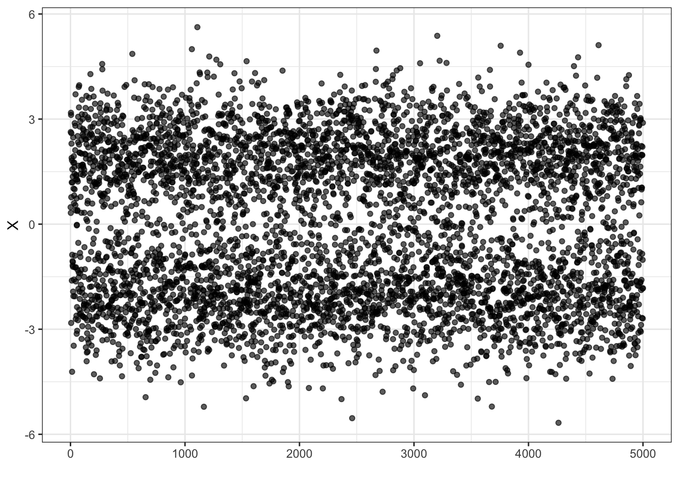
# Generate a random sample 
set.seed(123)  
# Generate empirical data
B <- rbinom(n, size = 1, prob = p)
Z1 <- rnorm(n, mean = mu1, sd = sigma1)
Z2 <- rnorm(n, mean = mu2, sd = sigma2)
x <- B*Z1 + (1-B)*Z2
# ======================================================================
# Perturb the true parameters 
par <- init_params <- true_params*runif(length(true_params), min = 0.8, max = 1.2)
abstol <- 1e-6 # absolute threshold tolerance for convergence 
maxit <- 1000 # maximum iteration 
match_moments = FALSE # match empirical moments for second distribution
# ======================================================================
# Number of observations 
n_ <- length(x)
# Empiric expectation 
e_x_emp = mean(x)
# Empiric variance 
v_x_emp = var(x)
# Empiric std. deviation  
sd_x_emp = sqrt(v_x_emp)

# Initialization 
log_likelihood <- 0
previous_log_likelihood <- -Inf
responsibilities <- matrix(0, nrow = n, ncol = 2)
previous_params <- par
# EM Routine 
for (iteration in 1:maxit) {
  # 1. E-step: Calculate the responsibilities
  for (i in 1:n_) {
    responsibilities[i, 1] <- previous_params[5] * dnorm(x[i], previous_params[1], previous_params[3])
    responsibilities[i, 2] <- (1 - previous_params[5]) * dnorm(x[i], previous_params[2], previous_params[4])
  }
  # Normalize the probabilities by row
  responsibilities <- responsibilities/rowSums(responsibilities)
  
  # 2. M-step: Update the parameters
  n1 <- sum(responsibilities[, 1])
  n2 <- sum(responsibilities[, 2])
  # A) First component 
  ## Means 
  mu1 <- sum(responsibilities[, 1] * x) / n1 # means 
  ## Std. deviations 
  sigma1 <- sqrt(sum(responsibilities[, 1] * (x - mu1)^2)/(n1-1)) # std. deviation  
  # B) Second component  
  if (match_moments) {
    # Match moments approach for (mu2, sigma2)
    # Means 
    mu2 <- (e_x_emp - p * mu1) / (1 - p)
    # Std- deviations
    sigma2 <- sqrt((v_x_emp - p * sigma1^2) / (1 - p) - p * (mu1 - mu2)^2)
  } else {
    # Means
    mu2 <- sum(responsibilities[, 2] * x) / n2 
    # Std. deviations
    sigma2 <- sqrt(sum(responsibilities[, 2] * (x - mu2)^2) / (n2 - 1))  
  }
  # C) Bernoulli probability 
  p <- n1 / n_

  # 3. Calculate the log-likelihood
  log_likelihood <- sum(log(rowSums(responsibilities*cbind(p * dnorm(x, mu1, sigma1), (1 - p) * dnorm(x, mu2, sigma2)))))
  
  # 4. Check for convergence
  if (abs(log_likelihood - previous_log_likelihood) < abstol) {
    break
  }
  # Update log-likelihood
  previous_log_likelihood <- log_likelihood
  # Update parameters 
  previous_params <- c(mu1, mu2, sigma1, sigma2, p)
}
# ======================================================================
# Output 
# Mixture classification
B_hat <- ifelse(responsibilities[, 1] > responsibilities[, 2], 1, 0)
x1_hat <- x[B_hat == 1]
x2_hat <- x[B_hat == 0]
# Optimal parameters 
par <- previous_params
# Theoretical moments 
e_x_th <- par[1]*par[5] + par[2]*(1-par[5])
sd_x_th <- sqrt(par[5]*(1-par[5])*(par[1] - par[2])^2 + par[3]^2*par[5] + par[4]^2*(1-par[5]))
# Empirical parameters 
par_hat <- c(mean(x1_hat), mean(x2_hat), sd(x1_hat), sd(x2_hat), mean(B_hat))
# Empirical moments 
e_x_hat <- par_hat[1]*par_hat[5] + par_hat[2]*(1-par_hat[5])
sd_x_hat <- sqrt(par_hat[5]*(1-par_hat[5])*(par_hat[1] - par_hat[2])^2 + par_hat[3]^2*par_hat[5] + par_hat[4]^2*(1-par_hat[5]))
# ======================================================================
# Dataset containing classified series 
data = dplyr::tibble(B = B_hat, x = x, x1 = x*B, x2 = x*(1-B))
# Dataset containing initial, optimal, empirical and true parameters 
params = tibble(param = c("mu1","mu2","sd1","sd2","p"), 
                init = init_params,
                opt = par, 
                hat = par_hat,
                true = true_params)
# Dataset containing empirical and theoretical moments series 
moments = tibble(statistic = c("Mean", "Std. Dev"), 
                 emp = c(e_x_emp, sd_x_emp), 
                 opt = c(e_x_th, sd_x_th), 
                 hat = c(e_x_hat, sd_x_hat))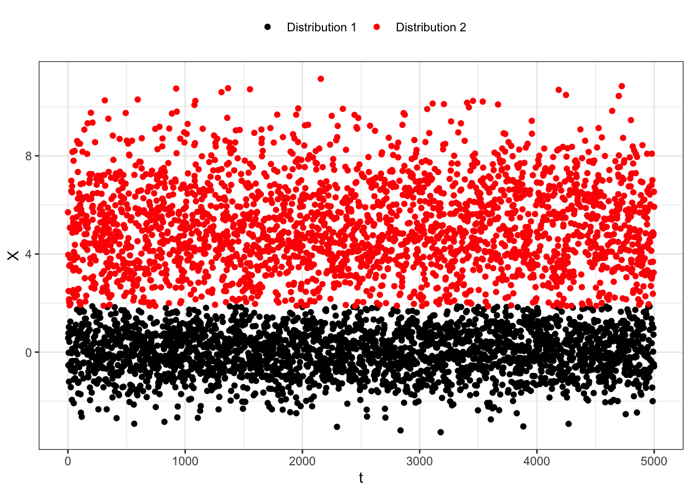

Table 31.3: Estimated Gaussian Mixture moments with EM

statistic	emp	opt	hat
Mean	2.516087	2.516087	2.516087
Std. Dev	2.958034	2.957904	2.957879

Figure 31.3: Classified simulated series with EM

31.5.4 Matrix moments matching

Proposition 31.7 Any finite K-component Gaussian mixture with finite moments admits a more parsimonious moment-matching approximation with only two-component Gaussian mixture. We start with the parameters of the mixture at time $t+h$ and we adjust them to match the first three moments of the multinomial mixture. The procedure ensures that the resulting distribution will have mean: $$\begin{array}{rl}& \mathbb{E}\{U_{t+h}\mid {\mathcal{F}}_t\}=\text{M}(t,0,h)\\ & \mathbb{V}\{U_{t+h}\mid {\mathcal{F}}_t\}=\text{S}(t,0,h)\\ & \mathbb{E}\{U_{t+h}\mid {\mathcal{F}}_t\}=\mathrm{\Omega }(t,0,h)\end{array}$$ where $$\mathrm{\Omega }(t,0,h)=\mathbb{E}\{U_{t+h}^3\mid {\mathcal{F}}_t\}=\sum _{j=0}^{h-1}\mathbb{E}\{{\psi }_{t+h-j}^3\mid {\mathcal{F}}_t\}\mathbb{E}\{u_{t+h-j}^3\}$$ In general, the variance and the skewness do not converge to a constant number for all $t$, but will depends on the skewness of the starting point at $t+1$ till the ending point at $t+h$ and needs to be recomputed each time. The parameters of the resulting mixture will be: $${\mu }_{1,t+h}^{\star }=\sqrt{{\mathrm{\Sigma }}_{t+h}}{\mu }_{1,t+h}{\mu }_{0,t+h}^{\star }=\sqrt{{\mathrm{\Sigma }}_{t+h}}{\mu }_{0,t+h}$$ and variances: $$\begin{array}{}\text{(31.9)}& \begin{array}{rl}{\sigma }_{1,t+h}^{\star 2}& =\frac{({\mathrm{\Sigma }}_{t+h}-p_{t+h}{\mu }_{1,t+h}^{\star 2}-(1-p_{t+h}){\mu }_{0,t+h}^{\star 2})\cdot 3{\mu }_{0,t+h}^{\star }(1-p_{t+h})-({\mathrm{\Omega }}_{t+h}-p_{t+h}{\mu }_{1,t+h}^{\star 3}-(1-p_{t+h}){\mu }_{0,t+h}^{\star 3})(1-p_{t+h})}{3p_{t+h}(1-p_{t+h})({\mu }_{0,t+h}^{\star }-{\mu }_{1,t+h}^{\star })}\end{array}\end{array}$$ and $$\begin{array}{}\text{(31.10)}& \begin{array}{rl}{\sigma }_{0,t+h}^{\star 2}& =\frac{({\mathrm{\Omega }}_{t+h}-p_{t+h}{\mu }_{1,t+h}^{3\ast }-(1-p_{t+h}){\mu }_{0,t+h}^{3\ast })p_{t+h}-3{\mu }_{1,t+h}^{\star }({\mathrm{\Sigma }}_{t+h}-p_{t+h}{\mu }_{1,t+h}^{\star 2}-(1-p_{t+h}){\mu }_{0,t+h}^{2\ast })p_{t+h}}{3p_{t+h}(1-p_{t+h})({\mu }_{0,t+h}^{\ast }-{\mu }_{1,t+h}^{\ast })}\end{array}\end{array}$$

Proof. Let’s consider the following approach. We start by fixing the mixture probabilities at time $t+h$, i.e. $p_{t+h}$. Then, we consider the means and variances parameters of the mixture at time $t+h$ free to vary and we adjust them to match the first three central moments of the true multinomial mixture with a two component Gaussian mixture. More precisely, let’s define: $$\begin{array}{}\text{(31.11)}& {\mu }_{i,t+h}^{\ast }={\mu }_{Y_i}(t,h)\text{,}{\sigma }_{i,t+h}^{2\ast }={\sigma }_{Y_i}^2(t,h)\end{array}$$ Recalling the central moments as in ?eq-proof-ut-moments we have that, with the parameters defined as in Equation 31.11, the resulting expected value and variance already matches the exact expectation and variance of the multinomial mixture. To improve the match between the two distributions, one can explicit also the third central moment, i.e. $${\omega }_{t+h}=(3{\sigma }_{1,t+h}^{2\ast }{\mu }_{1,t+h}^{\ast }+{\mu }_{1,t+h}^{3\ast }{p}_{t+h})+(3{\sigma }_{0,t+h}^{2\ast }{\mu }_{0,t+h}^{\ast }+{\mu }_{0,t+h}^{3\ast })(1-p_{t+h})$$ In this way, one can set a system to adjust the variances ${\sigma }_{i,t+h}^{\ast 2}$ such that the second and the third central moments of the Gaussian mixture with two components matches the ones of the multinomial mixture. More precisely, the third central moment of $y_{t+h}$ reads:
$${\kappa }_3\{y_{t+h}\mid {\mathcal{F}}_t\}=\sum _{j=s}^{h-1}\mathbb{E}\{{\psi }_{t+h-j}^3\mid {\mathcal{F}}_t\}\mathbb{E}\{u_{t+h-j}^3\}\text{.}$$ Let’s denote the target moments as: $${\mathrm{\Sigma }}_{t+h}={\kappa }_2\{y_{t+h}\mid {\mathcal{F}}_t\}{\mathrm{\Omega }}_{t+h}={\kappa }_3\{y_{t+h}\mid {\mathcal{F}}_t\}$$ and let’s represent the system in matrix form $$\underset{\mathbf{D}}{\underbrace{\left(\begin{array}{cc}{p}_{t+h}& 1-p_{t+h}\\ 3p_{t+h}{\mu }_{1,t+h}^{\ast }& 3(1-p_{t+h}{\mu }_{0,t+h}^{\ast })\end{array}\right)}}\underset{{\mathbf{\Sigma }}_{\mathbf{t}\mathbf{+}\mathbf{h}}^{\star }}{\underbrace{\left(\begin{array}{c}{\sigma }_{1,t+h}^{2\star }\\ {\sigma }_{0,t+h}^{2\star }\end{array}\right)}}=\underset{\mathbf{G}}{\underbrace{\left(\begin{array}{c}{\mathrm{\Sigma }}_{t+h}-p_{t+h}{\mu }_{1,t+h}^{2\ast }-(1-p_{t+h}){\mu }_{0,t+h}^{2\ast }\\ {\mathrm{\Omega }}_{t+h}-p_{t+h}{\mu }_{1,t+h}^{3\ast }-(1-p_{t+h}){\mu }_{0,t+h}^{2\ast }\end{array}\right)}}$$ The solution of the system has the form $\mathbf{D}{\mathrm{\Sigma }}^{\star }=\mathbf{G}⟺{\mathrm{\Sigma }}^{\star }={\mathbf{D}}^{-1}\mathbf{G}$. The determinant of the matrix $\mathbf{D}$ is different from zero only if ${\mu }_{1,t+h}^{\ast }\ne {\mu }_{0,t+h}^{\ast }$, i.e.  $$det(\mathbf{D})=3p_{t+h}(1-p_{t+h})({\mu }_{0,t+h}^{\ast }-{\mu }_{1,t+h}^{\ast })\text{.}$$ By applying Cramer’s rule the system can be solved explicitly for $i\in \{0,1\}$, i.e.  $$\begin{array}{}\text{(31.12)}& {\sigma }_{i,t+h}^{2\star }=\frac{det({\mathbf{D}}_i)}{det(\mathbf{D})}\end{array}$$ Where ${\mathbf{D}}_1$ is obtained by replacing the first column of $\mathbf{D}$ with the first column of $\mathbf{G}$, i.e. $${\mathbf{D}}_1=\left(\begin{array}{cc}{\mathrm{\Sigma }}_{t+h}-p_{t+h}{\mu }_{1,t+h}^{2\ast }-(1-p_{t+h}){\mu }_{0,t+h}^{2\ast }& 1-p_{t+h}\\ {\mathrm{\Omega }}_{t+h}-p_{t+h}{\mu }_{1,t+h}^{3\star }-(1-p_{t+h}){\mu }_{0,t+h}^{3\ast }& 3(1-p_{t+h}){\mu }_{0,t+h}^{\ast }\end{array}\right)$$ Then: $$\begin{array}{rl}det({\mathbf{D}}_1)& =({\mathrm{\Sigma }}_{t+h}-p_{t+h}{\mu }_{1,t+h}^{\star 2}-(1-p_{t+h}){\mu }_{0,t+h}^{\star 2})\cdot 3(1-p_{t+h}){\mu }_{0,t+h}^{\star }+\\ & -(1-p_{t+h})({\mathrm{\Omega }}_{t+h}-p_{t+h}{\mu }_{1,t+h}^{\star 3}-(1-p_{t+h}){\mu }_{0,t+h}^{\star 3})\end{array}$$ Similarly for the second component ${\mathbf{D}}_0$ is obtained by replacing the second column of $\mathbf{D}$ with the second column of $\mathbf{G}$, i.e. $${\mathbf{D}}_0=\left(\begin{array}{cc}{p}_{t+h}& {\mathrm{\Sigma }}_{t+h}-p_{t+h}{\mu }_{1,t+h}^{\star 2}-(1-p_{t+h}){\mu }_{0,t+h}^{\star 2}\\ 3p_{t+h}{\mu }_{1,t+h}^{\star }& {\mathrm{\Omega }}_{t+h}-p_{t+h}{\mu }_{1,t+h}^{\star 3}-(1-p_{t+h}){\mu }_{0,t+h}^{\star 3}\end{array}\right)$$ Then: $$\begin{array}{rl}det({\mathbf{D}}_0)& =p_{t+h}\cdot ({\mathrm{\Omega }}_{t+h}-p_{t+h}{\mu }_{1,t+h}^{\star 3}-(1-p_{t+h}){\mu }_{0,t+h}^{\star 3})+\\ & -3p_{t+h}{\mu }_{1,t+h}^{\star }\cdot ({\mathrm{\Sigma }}_{t+h}-p_{t+h}{\mu }_{1,t+h}^{\star 2}-(1-p_{t+h}){\mu }_{0,t+h}^{\star 2})\end{array}$$ Substituting and developing Equation 31.12, one obtain the explicit solutions of the system.