14  Introduction

Statistical modeling applies statistical methods to real-world data to give empirical content to relationships. It aims to quantify phenomena and develop models and test hypotheses, making it a crucial field for economic research, policy analysis, and decision-making. The aim of the statistical modeling is to study the (unknown) mechanism that generates the data, i.e., the Data Generating Process (DGP). The statistical model is a function that approximates the DGP.

14.1 The matrix of data

Let’s consider $n$ realizations defining a sample for $i=1,2,\dots ,n$. Suppose we have $p$ dependent variables and $k$ explanatory variables (also known as predictors). The data matrix for $\mathbf{X}$, the exogenous (regressors), is then composed as: $$\underset{n\times k}{\mathbf{X}}=\left(\begin{array}{cccccc}{x}_{1,1}& x_{1,2}& \dots & x_{1,j}& \dots & x_{1,k}\\ x_{2,1}& x_{2,2}& \dots & x_{2,j}& \dots & x_{2,k}\\ ⋮& ⋮& \ddots & ⋮& \ddots & ⋮\\ x_{n,1}& x_{n,2}& \dots & x_{n,j}& \dots & x_{n,k}\end{array}\right)=\left(\begin{array}{c}{\mathbf{x}}_1^{\mathrm{\top }}\\ {\mathbf{x}}_2^{\mathrm{\top }}\\ ⋮\\ {\mathbf{x}}_k^{\mathrm{\top }}\end{array}\right)\text{,}$$ where

• The i-th row contains the variables related to the $i$-th statistical unit (e.g., an individual, a firm, or a country).
• The j-th column contains all the observations related to the $j$-th variable.

The matrix $\mathbf{Y}$ represent the endogenous (dependent), i.e.  $$\underset{n\times p}{\mathbf{Y}}=\left(\begin{array}{cccccc}{y}_{1,1}& y_{1,2}& \dots & y_{1,j}& \dots & y_{1,p}\\ y_{2,1}& y_{2,2}& \dots & y_{2,j}& \dots & y_{2,p}\\ ⋮& ⋮& \ddots & ⋮& \ddots & ⋮\\ y_{n,1}& y_{n,2}& \dots & y_{n,j}& \dots & y_{n,p}\end{array}\right)=\left(\begin{array}{c}{\mathbf{y}}_1^{\mathrm{\top }}\\ {\mathbf{y}}_2^{\mathrm{\top }}\\ ⋮\\ {\mathbf{y}}_p^{\mathrm{\top }}\end{array}\right)\text{.}$$ Hence, the complete matrix of data $\mathbf{W}$ reads $$\begin{array}{}\text{(14.1)}& \underset{n\times (k+p)}{\mathbf{W}}=\left(\begin{array}{c}\mathbf{Y}\mathbf{X}\end{array}\right)=\left(\begin{array}{cccccc}{y}_{1,1}& \dots & y_{1,p}& x_{1,1}& \dots & x_{1,k}\\ ⋮& \ddots & ⋮& ⋮& \ddots & ⋮\\ y_{n,1}& \dots & y_{n,p}& x_{n,1}& \dots & x_{n,k}\end{array}\right)\text{.}\end{array}$$ In general, when $p=1$ then the model has only one equation to satisfy for $i=1,\dots ,n$, for example $$\begin{array}{}\text{(14.2)}& y_i=b_0+b_1{x}_{i,1}+b_2{x}_{i,2}+\cdots +b_k{x}_{i,k}+e_i\text{.}\end{array}$$ Otherwise, when $p>1$ there are more than one dependent variable and the model is composed by $p$-equations for $i=1,\dots ,n$, i.e. the same linear model with $p$ equations reads: $$\begin{array}{}\text{(14.3)}& \{\begin{array}{l}{y}_{i,1}=b_{0,1}+b_{1,1}{x}_{i,1}+b_{1,2}{x}_{i,2}+\cdots +b_{1,k}{x}_{i,k}+e_{i,1}\\ y_{i,2}=b_{0,2}+b_{2,1}{x}_{i,1}+b_{2,2}{x}_{i,2}+\cdots +b_{2,k}{x}_{i,k}+e_{i,2}\\ ⋮\\ y_{i,p}=b_{0,p}+b_{p,1}{x}_{i,1}+b_{p,2}{x}_{i,2}+\cdots +b_{p,k}{x}_{i,k}+e_{i,p}\end{array}\end{array}$$

14.2 Joint, conditional and marginals

Let’s consider the bi-dimensional random vector $\mathbf{W}$ in Equation 14.1 and let’s write the joint distribution of $\mathbf{X}$ and $\mathbf{Y}$, i.e.  $$\begin{array}{}\text{(14.4)}& \underset{\text{joint probability}}{\mathbb{P}(\mathbf{Y}\le \mathbf{y},\mathbf{X}\le \mathbf{x})}=\underset{\text{distribution function}}{F_{\mathbf{Y},\mathbf{X}}(\mathbf{y},\mathbf{x})}\text{.}\end{array}$$ In the continuous case, there exists a joint density $f_{\mathbf{Y},\mathbf{X}}(\mathbf{y},\mathbf{x})$ such that: $$\begin{array}{}\text{(14.5)}& F_{\mathbf{Y},\mathbf{X}}(\mathbf{y},\mathbf{x})={\int }_{-\mathrm{\infty }}^{\mathbf{x}}{\int }_{-\mathrm{\infty }}^{\mathbf{y}}{f}_{\mathbf{Y},\mathbf{X}}(\mathbf{y},\mathbf{x})d\mathbf{y}d\mathbf{x}\text{.}\end{array}$$ Moreover, from the joint distribution (Equation 14.4) it is possible to recover the marginals distributions, i.e.
$$\begin{array}{}\text{(14.6)}& \begin{array}{rl}& f_{\mathbf{Y}}(\mathbf{y})={\partial }_{\mathbf{y}}{F}_{\mathbf{Y},\mathbf{X}}(\mathbf{y},\mathbf{x})={\int }_{-\mathrm{\infty }}^{\mathrm{\infty }}{f}_{\mathbf{Y},\mathbf{X}}(\mathbf{y},\mathbf{x})d\mathbf{x}\\ & f_{\mathbf{X}}(\mathbf{x})={\partial }_{\mathbf{x}}{F}_{\mathbf{Y},\mathbf{X}}(\mathbf{y},\mathbf{x})={\int }_{-\mathrm{\infty }}^{\mathrm{\infty }}{f}_{\mathbf{Y},\mathbf{X}}(\mathbf{y},\mathbf{x})d\mathbf{y}\end{array}\end{array}$$

Then, given the marginals (Equation 14.6), it is possible to compute the unconditional moments, i.e.

1. First moment: $\mathbb{E}\{\mathbf{Y}\}={\int }_{-\mathrm{\infty }}^{\mathrm{\infty }}\mathbf{y}{f}_{\mathbf{Y}}(\mathbf{y})d\mathbf{y}$.
2. Second moment: $\mathbb{E}\{{\mathbf{Y}}^2\}={\int }_{-\mathrm{\infty }}^{\mathrm{\infty }}{\mathbf{y}}^2{f}_{\mathbf{Y}}(\mathbf{y})d\mathbf{y}$.
3. Variance: $\mathbb{V}\{\mathbf{Y}\}=\mathbb{E}\{{\mathbf{Y}}^2\}-\mathbb{E}\{\mathbf{Y}{\}}^2$.

Using the Bayes theorem (Theorem 6.2), from the joint distribution (Equation 14.4) it is possible to recover the conditional distribution, i.e
$$\begin{array}{}\text{(14.7)}& f_{\mathbf{Y}\mid \mathbf{X}}(\mathbf{y}\mid \mathbf{x})=\frac{f_{\mathbf{Y},\mathbf{X}}(\mathbf{y},\mathbf{x})}{f_{\mathbf{X}}(\mathbf{x})}\text{.}\end{array}$$ Given the conditional distributions, it is possible to compute the conditional moments, i.e. 

1. First moment: $\mathbb{E}\{\mathbf{Y}\mid \mathbf{X}\}={\int }_{-\mathrm{\infty }}^{\mathrm{\infty }}\mathbf{y}{f}_{\mathbf{Y}\mid \mathbf{X}}(\mathbf{y}\mid \mathbf{x})d\mathbf{y}$.
2. Second moment: $\mathbb{E}\{{\mathbf{Y}}^2\mid \mathbf{X}\}={\int }_{-\mathrm{\infty }}^{\mathrm{\infty }}{\mathbf{y}}^2{f}_{\mathbf{Y}\mid \mathbf{X}}(\mathbf{y}\mid \mathbf{x})d\mathbf{y}$.

Hence, from Equation 14.7 the joint density can be represented as the product of the conditional and the marginal, i.e.  $$\begin{array}{}\text{(14.8)}& \underset{\text{joint}}{f_{\mathbf{Y},\mathbf{X}}(\mathbf{y},\mathbf{x})}=\underset{\text{conditional}}{f_{\mathbf{Y}\mid \mathbf{X}}(\mathbf{y}\mid \mathbf{x})}\cdot \underset{\text{marginal}}{f_{\mathbf{X}}(\mathbf{x})}\text{.}\end{array}$$

Inference in a multivariate Gaussian model

Example 14.1 Let’s consider a Gaussian setup, i.e.  $${\mathbf{W}}^{\mathrm{\top }}=\left(\begin{array}{c}\mathbf{Y}\\ \mathbf{X}\end{array}\right)\sim \mathcal{N}(\left(\begin{array}{c}{\mathit{\mu }}_{\mathbf{Y}}\\ {\mathit{\mu }}_{\mathbf{X}}\end{array}\right),\left(\begin{array}{cc}{\mathbf{\Sigma }}_{\mathbf{Y}\mathbf{Y}}& {\mathbf{\Sigma }}_{\mathbf{Y}\mathbf{X}}\\ {\mathit{\mu }}_{\mathbf{X}\mathbf{Y}}& {\mathbf{\Sigma }}_{\mathbf{X}\mathbf{X}}\end{array}\right))$$ For a Gaussian setup if $(\mathbf{X}\mathbf{Y})$ are jointly normal, then the marginals are normal, i.e. $$\mathbf{Y}\sim \mathcal{N}({\mathit{\mu }}_{\mathbf{Y}},{\mathbf{\Sigma }}_{\mathbf{Y}\mathbf{Y}})\text{,}\mathbf{X}\sim \mathcal{N}({\mathit{\mu }}_{\mathbf{X}},{\mathbf{\Sigma }}_{\mathbf{X}\mathbf{X}})\text{.}$$ and also the conditionals distributions are normal, i.e.  $$\mathbf{Y}\mid \mathbf{X}\sim \mathcal{N}({\mathit{\mu }}_{\mathbf{Y}\mid \mathbf{X}},{\mathbf{\Sigma }}_{\mathbf{Y}\mathbf{Y}\mid \mathbf{X}})\text{,}\mathbf{X}\mid \mathbf{Y}\sim \mathcal{N}({\mathit{\mu }}_{\mathbf{X}\mid \mathbf{Y}},{\mathbf{\Sigma }}_{\mathbf{X}\mathbf{X}\mid \mathbf{Y}})\text{.}$$ and the conditional moments reads explicitly as: $$\begin{array}{rl}\mathbb{E}\{\mathbf{Y}\mid \mathbf{X}\}& ={\mathit{\mu }}_{\mathbf{Y}\mid \mathbf{X}}=\\ & ={\mathit{\mu }}_{\mathbf{Y}}+{\mathbf{\Sigma }}_{\mathbf{Y}\mathbf{X}}\cdot {\mathbf{\Sigma }}_{\mathbf{X}\mathbf{X}}^{-1}(\mathbf{X}-{\mathit{\mu }}_{\mathbf{X}})=\\ & ={\mathit{\mu }}_{\mathbf{Y}}-{\mathbf{\Sigma }}_{\mathbf{Y}\mathbf{X}}\cdot {\mathbf{\Sigma }}_{\mathbf{X}\mathbf{X}}^{-1}{\mathit{\mu }}_{\mathbf{X}}+{\mathbf{\Sigma }}_{\mathbf{Y}\mathbf{X}}\cdot {\mathbf{\Sigma }}_{\mathbf{X}\mathbf{X}}^{-1}\mathbf{X}=\\ & ={\mathit{\mu }}_{\mathbf{Y}}-{\mathbf{b}}_{\mathbf{Y}\mid \mathbf{X}}{\mathit{\mu }}_{\mathbf{X}}+{\mathbf{b}}_{\mathbf{Y}\mid \mathbf{X}}\mathbf{X}=\\ & ={\mathbf{a}}_{\mathbf{Y}\mid \mathbf{X}}+{\mathbf{b}}_{\mathbf{Y}\mid \mathbf{X}}\mathbf{X}\end{array}$$ and $$\mathbb{V}\{\mathbf{Y}\mid \mathbf{X}\}={\mathbf{\Sigma }}_{\mathbf{Y}\mathbf{Y}}-{\mathbf{\Sigma }}_{\mathbf{Y}\mathbf{X}}\cdot {\mathbf{\Sigma }}_{\mathbf{X}\mathbf{X}}^{-1}{\mathbf{\Sigma }}_{\mathbf{Y}\mathbf{X}}\text{.}$$ In this setup the parameters are:

• Joint distribution, $\mathit{\theta }=\{{\mathit{\mu }}_{\mathbf{Y}},{\mathit{\mu }}_{\mathbf{X}},{\mathbf{\Sigma }}_{\mathbf{X}\mathbf{X}},{\mathbf{\Sigma }}_{\mathbf{X}\mathbf{Y}},{\mathbf{\Sigma }}_{\mathbf{Y}\mathbf{Y}}\}$.
• Conditional distribution, ${\mathit{\lambda }}_1=\{{\mathbf{a}}_{\mathbf{Y}\mid \mathbf{X}},{\mathbf{b}}_{\mathbf{Y}\mid \mathbf{X}},{\mathbf{\Sigma }}_{\mathbf{Y}\mathbf{Y}\mid \mathbf{X}}\}$.
• Marginal distribution, ${\mathit{\lambda }}_2=\{{\mathit{\mu }}_{\mathbf{X}},{\mathbf{\Sigma }}_{\mathbf{X}\mathbf{X}}\}$.

Noting that ${\mathit{\lambda }}_1$ is a function of $\mathit{\theta }$, i.e. $\tau =f({\mathit{\lambda }}_1)$ in the Gaussian case it is possible to prove that ${\mathit{\lambda }}_1$ and ${\mathit{\lambda }}_2$ are free to vary. Hence, imposing restrictions on ${\mathit{\lambda }}_1$ do not impose restrictions on ${\mathit{\lambda }}_2$. In general, if the parameters of interest are a function of the conditional distribution and ${\mathit{\lambda }}_1$ and ${\mathit{\lambda }}_2$ are free to vary, then the inference can be done without losing of information considering the conditional model. In this case we say that $\mathbf{X}$ is weakly exogenous for $\tau =f({\mathit{\lambda }}_1)$.

14.3 Conditional expectation model

Let’s consider a very general conditional expectation model with $p=1$, of which the linear models are a special case. In matrix notation it can be written as: $$\begin{array}{}\text{(14.9)}& \mathbf{y}=\mathbb{E}\{\mathbf{y}\mid \mathbf{X}\}+\mathbf{e}\text{,}\end{array}$$ where the conditional expectation errors are defined as: $$\begin{array}{}\text{(14.10)}& \mathbf{e}=\mathbf{y}-\mathbb{E}\{\mathbf{y}\mid \mathbf{X}\}\text{.}\end{array}$$ Then, in general the unconditional expectation of the residuals $\mathbf{e}$ and the covariance between the residuals and the regressors are zero, i.e. $$\mathbb{E}\{\mathbf{e}\}=0,\mathbb{E}\{\mathbf{e}\mathbf{X}\}=0\text{.}$$ Moreover, the conditional expectation error is orthogonal to any transformation of the conditioning variables. Consider a more general setup, i.e.  $$\begin{array}{}\text{(14.11)}& \mathbf{y}=\mathbb{E}\{\mathbf{y}\mid \mathbf{X}\}+\mathbf{e},\mathbb{E}\{\mathbf{y}\mid \mathbf{X}\}=g(\mathbf{X})\text{,}\end{array}$$ we have that
$$\mathbb{E}\{\mathbf{e}g(\mathbf{X})\}=0\text{.}$$

In a conditional expectation model the residuals and the regressors are uncorrelated

Proof. Let’s start the unconditional expectation of the residuals defined in Equation 14.9, i.e.  $$\begin{array}{rl}\mathbb{E}\{\mathbf{e}\}& =\mathbb{E}\{\mathbf{y}-\mathbb{E}\{\mathbf{y}\mid \mathbf{X}\}\}=\\ & =\mathbb{E}\{\mathbf{y}\}-\mathbb{E}\{\mathbb{E}\{\mathbf{y}\mid \mathbf{X}\}\}=\\ & =\mathbb{E}\{\mathbf{y}\}-\mathbb{E}\{\mathbf{y}\}=0\end{array}$$ Then, let’s compute the expected value of between the residuals and the regressors, i.e.  $$\mathbb{E}\{\mathbf{e}\}=0⟹\mathbb{C}v\{\mathbf{e},\mathbf{X}\}=\mathbb{E}\{\mathbf{e}\mathbf{X}\}$$ For simplicity let’s assume that $\mathbf{X}$ can takes only values in $\{0,1\}$. Applying the tower property of conditional expectation one obtain: $$\begin{array}{rl}\mathbb{E}\{\mathbf{e}\mathbf{X}\}& =\mathbb{E}\{\mathbb{E}\{\mathbf{e}\mathbf{X}\mid \mathbf{X}\}\}=\\ & =\mathbb{E}\{\mathbf{e}\mathbf{X}\mid \mathbf{X}=0\}\mathbb{P}(\mathbf{X}=0)+\mathbb{E}\{\mathbf{e}\mathbf{X}\mid \mathbf{X}=1\}\mathbb{P}(\mathbf{X}=1)=\\ & =\mathbb{E}\{\mathbf{e}\mathbf{X}\mid \mathbf{X}=1\}\mathbb{P}(\mathbf{X}=1)\end{array}$$ Then, let’s substitute $\mathbf{e}$ from Equation 14.9 and $\mathbf{X}$ with $1$, i.e. $$\begin{array}{rl}\mathbb{E}\{\mathbf{e}\mathbf{X}\}& =\mathbb{E}\{(\mathbf{y}-\mathbb{E}\{\mathbf{y}\mid \mathbf{X}\})\mathbf{X}\mid \mathbf{X}=1\}\mathbb{P}(\mathbf{X}=1)=\\ & =\mathbb{E}\{\mathbf{y}\mid \mathbf{X}=1\}\mathbb{P}(\mathbf{X}=1)-\mathbb{E}\{\mathbb{E}\{\mathbf{y}\mid \mathbf{X}\}\mid \mathbf{X}=1\}\mathbb{P}(\mathbf{X}=1)=\\ & =\mathbb{E}\{\mathbf{y}\mid \mathbf{X}=1\}\mathbb{P}(\mathbf{X}=1)-\mathbb{E}\{\mathbf{y}\mid \mathbf{X}=1\}\mathbb{P}(\mathbf{X}=1)=0\end{array}$$ For a general transformation of the regressors as in Equation 14.11, the covariance is computed as: $$\begin{array}{rl}\mathbb{E}\{\mathbf{e}g(\mathbf{X})\}& =\mathbb{E}\{\mathbb{E}\{\mathbf{e}g(\mathbf{X})\mid \mathbf{X}\}\}=\\ & =\mathbb{E}\{g(\mathbf{X})\mathbb{E}\{\mathbf{e}\mid \mathbf{X}\}\}=\\ & =\mathbb{E}\{g(\mathbf{X})\mathbb{E}\{\mathbf{y}-\mathbb{E}\{\mathbf{y}\mid \mathbf{X}\}\mid \mathbf{X}\}\}=\\ & =\mathbb{E}\{g(\mathbf{X})[\mathbb{E}\{\mathbf{y}\mid \mathbf{X}\}-\mathbb{E}\{\mathbf{y}\mid \mathbf{X}\}]\}=0\end{array}$$

14.4 Uniequational linear models

Let’s consider an uni-equational linear model, i.e. with $p=1$ in (Equation 14.2), is expressed in compact matrix notation as: $$\begin{array}{}\text{(14.12)}& \mathbf{y}=\mathbf{X}\mathbf{b}+\mathbf{e}\text{,}\end{array}$$ where $\mathbf{b}$ and $\mathbf{e}$ represent the true parameters and residuals in population. Let’s consider a sample of $n$-observations extracted from a population, then the matrix of the regressors $\mathbf{X}$ reads $$\underset{n\times k}{\mathbf{X}}=\left(\begin{array}{ccc}{x}_{1,1}& \dots & x_{1,k}\\ ⋮& & ⋮\\ x_{n,1}& \dots & x_{n,k}\end{array}\right)=\left(\begin{array}{c}{\mathbf{x}}_1^{\mathrm{\top }}\\ ⋮\\ {\mathbf{x}}_k^{\mathrm{\top }}\end{array}\right)\text{,}$$ while the vectors of dependent variable and of the residuals reads $$\underset{n\times 1}{\mathbf{y}}=\left(\begin{array}{c}{y}_1\\ ⋮\\ y_p\end{array}\right)\text{,}\underset{n\times 1}{\mathbf{e}}=\left(\begin{array}{c}{e}_1\\ ⋮\\ e_n\end{array}\right)\text{.}$$ Hence, the matrix of data $\mathbf{W}$ is composed by: $$\begin{array}{}\text{(14.13)}& \underset{n\times (k+1)}{\mathbf{W}}=\left(\begin{array}{c}\mathbf{y}\mathbf{X}\end{array}\right)=\left(\begin{array}{cccc}{y}_1& x_{1,1}& \dots & x_{1,k}\\ ⋮& ⋮& \ddots & ⋮\\ y_n& x_{n,1}& \dots & x_{n,k}\end{array}\right)\text{.}\end{array}$$

14.4.1 Estimators of b

Let’s denote with ${\mathrm{\Theta }}_{\mathbf{b}}$ the parameter space, i.e. ${\mathrm{\Theta }}_{\mathbf{b}}\subset {\mathbb{R}}^k$, and with $Q$ an estimator function of the unknown true parameter $\mathbf{b}\in {\mathrm{\Theta }}_{\mathbf{b}}$. Then, the function $Q$ defines an estimator of $\mathbf{b}$, meaning it is a function that takes the matrix of data as input and returns a vector of parameters within ${\mathrm{\Theta }}_{\mathbf{b}}$ as output: $$Q:\mathbf{W}⟶{\mathrm{\Theta }}_{\mathbf{b}},\text{such that}Q(\mathbf{W})=\hat{\mathbf{b}}\in {\mathrm{\Theta }}_{\mathbf{b}}\text{,}$$ where $\hat{\mathbf{b}}$ is an estimates of the true population’s parameter $\mathbf{b}$. Then, the fitted values $\hat{\mathbf{y}}$ are a function of the estimate and are defined as: $$\begin{array}{}\text{(14.14)}& \hat{\mathbf{y}}=\mathbf{X}\hat{\mathbf{b}}\text{.}\end{array}$$ Consequently, the fitted residuals, which measure the discrepancies between the observed and the fitted values, are also a function of $\hat{\mathbf{b}}$, i.e. $$\begin{array}{}\text{(14.15)}& \mathbf{e}(\hat{\mathbf{b}})=\mathbf{y}-\hat{\mathbf{y}}=\mathbf{y}-\mathbf{X}\hat{\mathbf{b}}\text{.}\end{array}$$

Different optimal estimators of $\mathbf{b}$

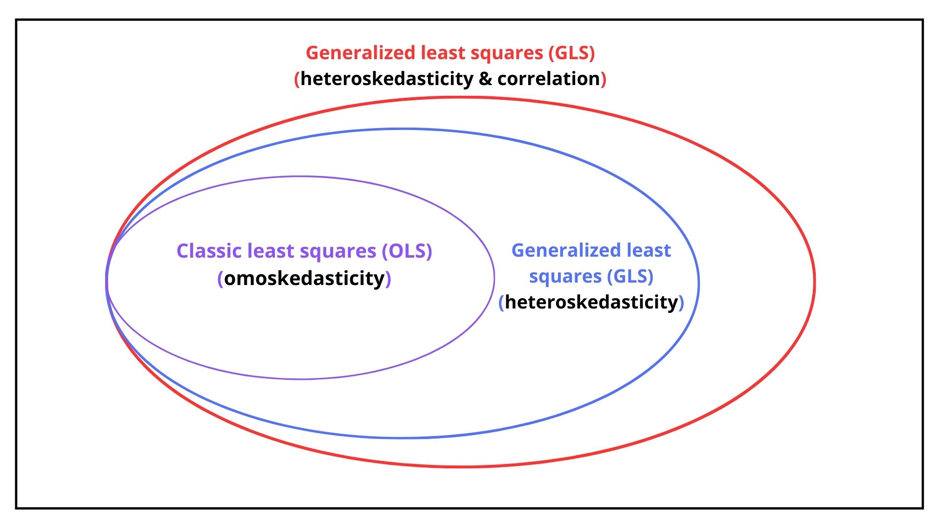
As we will see in Chapter 15, the assumptions on the variance of the residuals determines the optimal estimator of $\mathbf{b}$. In general, the residuals could be

1. omoskedastic: the residuals are uncorrelated and their variance is equal for each observation.
2. heteroskedastic: the residuals are uncorrelated and their variance is difference for each observation.
3. autocorrelated: the residuals are correlated and their variance is equal and their variance is difference for each observation.

As shown in Figure 14.1, depending on the assumption (1,2 or 3) the optimal estimator of $\mathbf{b}$ is obtained with Ordinary Last Square for case 1, while Generalized Last Square for case 2 and 3.

Figure 14.1: Different classes of estimator for linear models.

For example, if the residuals are autocorrelated, then their conditional variance-covariance matrix in matrix notation reads $$\underset{n\times n}{\mathbf{\Sigma }}=\mathbb{V}\{\mathbf{e}{\mathbf{e}}^{\mathrm{\top }}\mid \mathbf{X}\}=\mathbb{E}\{\mathbf{e}{\mathbf{e}}^{\mathrm{\top }}\mid \mathbf{X}\}\text{.}$$ More explicitly,
$$\begin{array}{}\text{(14.16)}& \underset{n\times n}{\mathbf{\Sigma }}=\left(\begin{array}{cccc}{e}_1^2& e_1{e}_2& \dots & e_1{e}_n\\ e_2{e}_1& e_2^2& \dots & e_2{e}_n\\ ⋮& ⋮& & ⋮\\ e_n{e}_1& e_n{e}_2& \dots & e_n^2\end{array}\right)=\left(\begin{array}{cccc}{\sigma }_1^2& {\sigma }_{1,2}& \dots & {\sigma }_{1,n}\\ {\sigma }_{2,1}& {\sigma }_2^2& \dots & {\sigma }_{2,n}\\ ⋮& ⋮& & ⋮\\ {\sigma }_{n,1}& {\sigma }_{n,2}& \dots & {\sigma }_n^2\end{array}\right)\text{.}\end{array}$$ Since the matrix $\mathbf{\Sigma }$ is symmetric the number of unique values (free elements) are given by $n$ variances and $\frac{n(n-1)}{2}$ covariances, i.e. $$n+\frac{n(n-1)}{2}=\frac{2n+n^2-n}{2}=\frac{n+n^2}{2}=\frac{n(n+1)}{2}\text{.}$$