25  Normality tests

library(dplyr) 
library(ggplot2)
library(knitr)

Tests of normality are statistical inference procedures designed to test that the underlying distribution of a random variable is normally distributed. There is a long history of these tests, and there are a plethora of them available for use, i.e. Jarque and Bera (1980), D’Agostino and Pearson (1973), Ralph B. D’agostino and Jr. (1990). Such kind of tests are based on the comparison of the sample skewness and kurtosis with the skewness and kurtosis of a normal distribution, hence their estimation is crucial.

skewness <- function(x, na.rm = FALSE){
  e_x <- mean(x, na.rm = na.rm)
  sd_x <- sd(x, na.rm = na.rm)
  mean((x - e_x)^3, na.rm = na.rm)/(sd_x^3)
}

kurtosis <- function(x, na.rm = FALSE, excess = TRUE){
  e_x <- mean(x, na.rm = na.rm)
  sd_x <- sd(x, na.rm = na.rm)
  mean((x - e_x)^4, na.rm = na.rm)/(sd_x^4) - ifelse(excess, 3, 0)
}

Proposition 25.1 (\(\color{magenta}{\textbf{Jarque-Brera test}}\))
Let’s consider an IID Gaussian sample with unknown means \(\mu\) and unknown variance \(\sigma^2\), i.e.  \[ \mathbf{X}_{n} \sim \mathcal{N}(\mu, \sigma^2) \text{,} \] Standardizing the skewness and kurtosis under \[ \mathcal{H}_0: \beta_1(\mathbf{X}_n) = 0, \, \beta_2(\mathbf{X}_n) = 3 \text{,} \] we have that asymptotically \[ \begin{aligned} {} & Z_1(\mathbf{X}_n) = \sqrt{n} \frac{b_1(\mathbf{X}_n)}{\sqrt{6}} && \underset{n \to \infty}{\overset{\text{d}}{\longrightarrow}} \mathcal{N}\left(0, 1\right) \text{,} \\ & Z_2(\mathbf{X}_n) = \sqrt{n} \frac{b_2(\mathbf{X}_n)-3}{\sqrt{24}} && \underset{n \to \infty}{\overset{\text{d}}{\longrightarrow}} \mathcal{N}\left(0, 1\right) \text{,} \end{aligned} \tag{25.1}\] where \(b_1\) reads as in Equation 10.12, \(b_2\) as in Equation 10.16 and it is possible to prove that the statistics \(Z_1(\mathbf{X}_n)\) and \(Z_2(\mathbf{X}_n)\) are independent.

Hence, since the sum of two independent standard normal squared random variables follows a \(\chi^{2}(2)\) distribution with 2 degrees of freedom, the Jarque-Brera statistic is obtained as \[ \text{JB}(\mathbf{X}_n) = Z_1(\mathbf{X}_n)^2 + Z_2(\mathbf{X}_n)^2 \underset{n \to \infty}{\overset{\text{d}}{\longrightarrow}} \chi^{2}(2) \text{.} \]

However, if \(n\) is small the \(\text{JB}(\mathbf{X}_n)\) over-reject the null hypothesis \(\mathcal{H}_0\), i.e. type I error.

Example: Jarque-Brera test

Example 25.1  

# =============== Setups =============== 
n <- 50 # number of simulations 
set.seed(1) # random seed 
ci <- 0.05 # confidence level 
# ======================================
# Simulated variable 
x <- rnorm(n, 0, 1)
# Sample skewness
b1 <- skewness(x)
# Sample kurtosis 
b2 <- kurtosis(x, excess = F)
# JB-statistic test
JB <- n*(b1^2/6 + (b2 - 3)^2/24)
# JB-test p-value 
pvalue <-  1 - pchisq(JB, df = 2)
# JB-test critic value at 95%
z_lim <- qchisq(1-ci, 2)

Figure 25.1: Jarque-Brera test for normality with a simulated Normal sample of 50 observations with \(\alpha = 0.05\).

Proposition 25.2 (\(\color{magenta}{\textbf{Urzua-Jarque-Brera test}}\))
Substituting in the JB-statistics from Equation 25.1 the exact sample moments of the skewness and kurtosis of a Normal sample instead the asymptotic moments, one obtain the UJB-test (see Urzúa (1996)), i.e.  \[ \begin{aligned} {} & \tilde{Z}_1(\mathbf{X}_n) = \frac{b_1(\mathbf{X}_n)}{\sqrt{\mathbb{V}\{b_1(\mathbf{X}_n)\}}} && \underset{n \to \infty}{\overset{\text{d}}{\longrightarrow}} \mathcal{N}\left(0, 1\right) \text{,} \\ & \tilde{Z}_2(\mathbf{X}_n) = \frac{b_2(\mathbf{X}_n) - \mathbb{E}\{b_2(\mathbf{X}_n)\}}{\sqrt{\mathbb{V}\{b_2(\mathbf{X}_n)\}}} && \underset{n \to \infty}{\overset{\text{d}}{\longrightarrow}} \mathcal{N}\left(0, 1\right) \text{,} \end{aligned} \tag{25.2}\] where the exact moments \(\mathbb{V}\{b_1(\mathbf{X}_n)\}\) (Equation 10.14), \(\mathbb{E}\{b_2(\mathbf{X}_n)\}\) (Equation 10.18) and \(\mathbb{V}\{b_2(\mathbf{X}_n)\}\) (Equation 10.19).

Hence, the Urzua-Jarque-Brera statistic adjusted for small samples is distributed asymptotically as a \(\chi^2(2)\), i.e.  \[ \text{UJB}(\mathbf{X}_n) = \tilde{Z}_1(\mathbf{X}_n)^2 + \tilde{Z}_2(\mathbf{X}_n)^2 \underset{n \to \infty}{\overset{\text{d}}{\longrightarrow}} \chi^{2}(2) \text{.} \]

Example: Urzua-Jarque-Brera test

Example 25.2  

# =============== Setups =============== 
n <- 50 # number of simulations 
set.seed(1) # random seed 
ci <- 0.05 # confidence level 
# ======================================
# Simulated variable 
x <- rnorm(n, 0, 1)
# Sample skewness
b1 <- skewness(x)
# Skewness's variance
v_b1 <- (6*(n-2))/((n+1)*(n+3))
# Statistic for skewness
Z1 <- b1/sqrt(v_b1)
# Sample kurtosis 
b2 <- kurtosis(x, excess = F)
# Kurtosis's expected value
e_b2 <- (3*(n-1))/(n+1)
# Kurtosis's variance
v_b2 <- (24*n*(n-2)*(n-3))/((n+1)^2*(n+3)*(n+5))
# Statistic for kurtosis
Z2 <- (b2-e_b2)/sqrt(v_b2)
# UJB-statistic test
UJB <- Z1^2 + Z2^2
# UJB p-value 
pvalue <-  1 - pchisq(UJB, df = 2)
# UJB critic value at 95%
z_lim <- qchisq(1-ci, 2)

Figure 25.2: Urzua-Jarque-Brera test for normality with a simulated Normal sample of 50 observations with \(\alpha = 0.05\).

25.1 D’Agostino skewness test

Starting from the statistic \(\tilde{Z}_1(\mathbf{X}_n)\) (Equation 25.2), let’s compute the fourth standardized moment of \(b_1\), i.e. \[ \beta_2(b_1) = \frac{3 (n^2 + 27n -70)(n+1)(n+3)}{(n-2)(n+5)(n+7)(n+9)} \text{,} \] Then, D’Agostino and Pearson (1973) proposed a statistic test for the skewness, defined as \[ Z_1^{\ast}(\mathbf{X}_n) = \delta \log \left\{\frac{\tilde{Z}_1(\mathbf{X}_n)}{\alpha} + \sqrt{\left(\frac{\tilde{Z}_1(\mathbf{X}_n)}{\alpha}\right)^2 + 1}\right\} \tag{25.3}\] where \[ \begin{aligned} {} & W^2 = \sqrt{2 \beta_2(b_1) - 1 } -1 \text{,} \\ & \delta = \frac{1}{\sqrt{\ln(W)}} \text{,} \\ & \alpha = \sqrt{\frac{2}{W^2 - 1}} \text{,} \end{aligned} \] and \(Z_1^{\ast}(\mathbf{X}_n) \sim \mathcal{N}(0,1)\). Notably, a more compact and equivalent expression reads \[ Z_1^{\ast}(\mathbf{X}_n) = \delta \sinh^{-1}\left( \frac{\tilde{Z}_1(\mathbf{X}_n)}{\alpha}\right) \text{.} \]

Example: D’Agostino test

Example 25.3  

# =============== Setups =============== 
n <- 20 # number of simulations 
set.seed(1) # random seed 
ci <- 0.05 # confidence level 
# ======================================
# Simulated variable 
x <- rnorm(n, 0, 1)
# Sample skewness
b1 <- skewness(x)
# Skewness's variance
v_b1 <- (6*(n-2))/((n+1)*(n+3))
# Statistic for skewness
Z1 <- b1/sqrt(v_b1)
# Test for Skewness 
beta2_b1 <- (3*(n^2 + 27*n - 70)*(n+1)*(n+3))/((n-2)*(n+5)*(n+7)*(n+9))
W2 <- sqrt(2*beta2_b1 - 1) - 1
delta <- 1/sqrt(log(sqrt(W2)))
alpha <- sqrt(2/(W2 - 1))
# Test for skewness
Z_ast_b1 <- delta*asinh(Z1/alpha)
# UJB p-value 
pvalue <- 1 - pnorm(Z_ast_b1, lower.tail = TRUE)
# UJB critic value at 95%
z_lim <- qnorm(1-ci/2)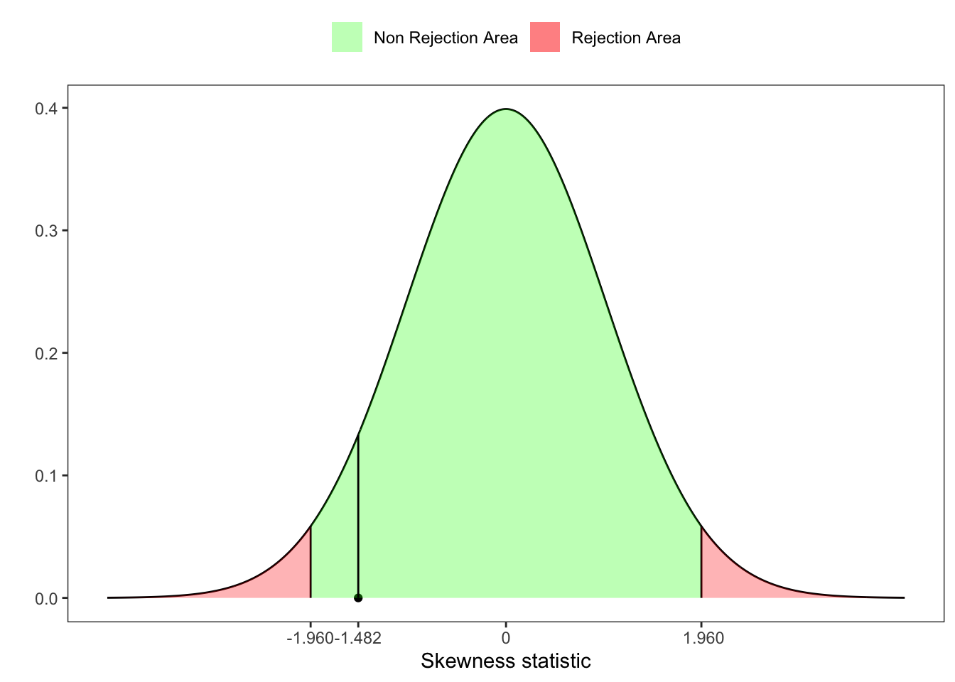

Figure 25.3: Skewness test with a simulated Normal sample of 50 observations with \(\alpha = 0.05\).

25.2 Anscombe Kurtosis test

Starting from the statistic \(\tilde{Z}_2(\mathbf{X}_n)\) (Equation 25.2), let’s compute the third standardized moment of \(b_2\): \[ \beta_1(b_2) = \frac{6(n^2 - 5n + 2)}{(n+7)(n+9)}\sqrt{\frac{6(n+3)(n+5)}{n(n-2)(n-3)}} \text{,} \] Then, Anscombe and Glynn (1983) proposed a statistic test for the kurtosis, defined as \[ Z_2^{\ast}(\mathbf{X}_n) = \sqrt{\frac{9A}{2}}\left(1 - \frac{2}{9A} - \left[\frac{1 - 2/A}{1 + \tilde{Z}_2(\mathbf{X}_n) \sqrt{2/(A - 4)} } \right]^{1/3} \right) \text{,} \tag{25.4}\] where \[ A = 6 + \frac{8}{\beta_1(b_2)} \left[\frac{2}{\beta_1(b_2)} + \sqrt{1 + \frac{4}{\beta_1(b_2)}}\right] \text{,} \] and \(Z_2^{\ast}(\mathbf{X}_n) \sim \mathcal{N}(0,1)\).

Example: Anscombe Kurtosis test

Example 25.4  

# =============== Setups =============== 
n <- 50 # number of simulations 
set.seed(1) # random seed 
ci <- 0.05 # confidence level 
# ======================================
# Simulated variable 
x <- rnorm(n, 0, 1)
# Sample kurtosis 
b2 <- kurtosis(x, excess = F)
# Kurtosis's expected value
e_b2 <- (3*(n-1))/(n+1)
# Kurtosis's variance
v_b2 <- (24*n*(n-2)*(n-3))/((n+1)^2*(n+3)*(n+5))
# Statistic for kurtosis
Z2 <- (b2-e_b2)/sqrt(v_b2)
# Test for Skewness 
beta1_b2 <- (6*(n^2 - 5*n + 2))/((n+7)*(n+9))*sqrt((6*(n+3)*(n+5))/(n*(n-2)*(n-3)))
A <- 6 + (8/beta1_b2)*(2/beta1_b2 + sqrt(1 + 4/(beta1_b2^2)))
# Test for kurtosis
Z_ast_b2 <- sqrt((9*A)/2) *(1 - 2/(9*A) - ((1 - 2/A)/(1 + Z2*sqrt(2/(A-4))))^(1/3))
# p-value 
pvalue <- 1 - pnorm(Z_ast_b2, lower.tail = TRUE)
# UJB critic value at 95%
z_lim <- qnorm(1-ci/2)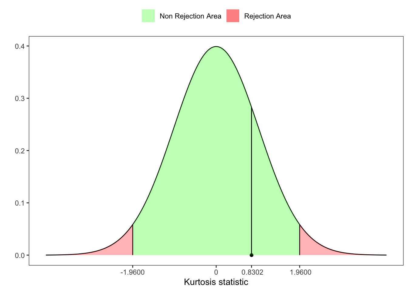

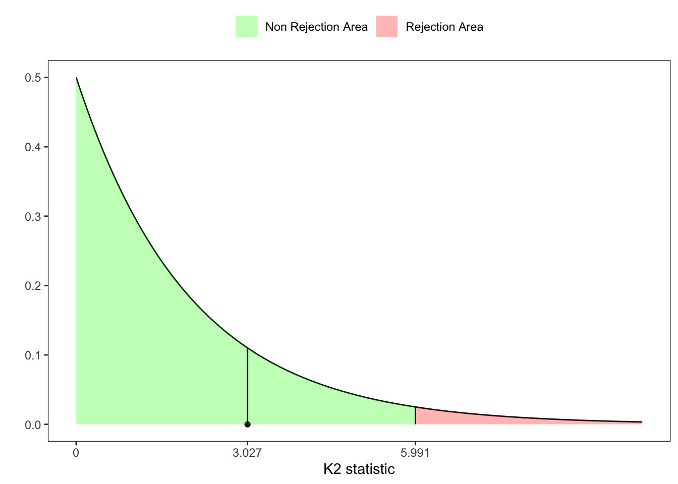
Figure 25.4: Kurtosis test with a simulated Normal sample of 50 observations with \(\alpha = 0.05\).

25.3 D’Agostino-Pearson \(K^2\) test

Following a same idea as in JB and UJB test, Ralph B. D’agostino and Jr. (1990) proposed an alternative omnibus test for Normality based on the statistics \(Z_1^{\ast}(\mathbf{X}_n)\) (Equation 25.3) and \(Z_2^{\ast}(\mathbf{X}_n)\) (Equation 25.4), i.e.  \[ \text{K}^2(\mathbf{X}_n) = (Z_1^{\ast}(\mathbf{X}_n))^2 + (Z_2^{\ast}(\mathbf{X}_n))^2 \sim \chi^2(2) \text{.} \]

Example: \(K^2\)-test

Example 25.5  

# K2-statistic test
K2 <- Z_ast_b1^2 + Z_ast_b2
# p-value 
pvalue <-  1 - pchisq(K2, df = 2)
# critic value at 95%
z_lim <- qchisq(1-ci, 2)

Figure 25.5: Agostino normality test with a simulated Normal sample of 50 observations with \(\alpha = 0.05\).

25.4 Kolmogorov-Smirnov test

The Kolmogorov–Smirnov test can be used to verify whether a samples is drawn from a reference distribution. In the case of q sample with dimension \(n\), the KS statistic is defined as: \[ \text{KS}_{n} = \underset{\forall x}{\sup}|\hat{F}_{\mathbf{X}_n} - F(x)| \text{,} \tag{25.5}\] where \(\hat{F}_n\) denotes the empirical distribution (Equation 23.4). The test statistic \(\text{KS}_{n}\) follows the Kolmogorov distribution \(F_{\text{KS}}\) defined as follows \[ F_{\text{KS}}(\sqrt{n}\cdot \text{KS}_{n} < x) = 1 - 2 \sum_{k = 1}^{\infty} (-1)^{k-1} e^{-2k^2x^2} \text{.} \]

# Infinite sum function
# k: approximation for infinity 
inf_sum <- function(x, k = 100){
  isum <- 0
  for(i in 1:k){
    isum <- isum + 2*(-1)^(i-1)*exp(-2*(x^2)*(i^2))
  }
  isum
}
# Kolmogorov distribution function  
pks <- function(x, k = 100){
  p <- c()
  for(i in 1:length(x)){
    p[i] <- 1-inf_sum(x[i], k = k)
  }
  p
}
# Kolmogorov quantile function  
qks <- function(p, k = 100){
  loss <- function(x, p){
    (pks(x, k = k) - p)^2
  }
  x <- c()
  for(i in 1:length(p)){
    x[i] <- optim(par = 2, method = "Brent", lower = 0, upper = 10, fn = loss, p = p[i])$par
  }
  x
}

The null distribution of this statistic is calculated under the null hypothesis that the sample is drawn from the reference distribution \(F\), i.e. \[ \begin{aligned} {} & \mathcal{H}_0: \hat{F}_{\mathbf{X}_n}(X) = F(X) \text{,} \\ & \mathcal{H}_1: \hat{F}_{\mathbf{X}_n}(X) \neq F(X) \text{.} \end{aligned} \] On large samples, \(\mathcal{H}_0\) is rejected at a given confidence level \(\alpha\) if: \[ \sqrt{n} \cdot \text{KS}_{n} > F_{KS}^{-1}(F_{\text{KS}}(\sqrt{n} \cdot \text{KS}_{n} < q_{\alpha})) \text{,} \] where \(q_{\alpha}\) represents the critical value and \(F_{\text{KS}}^{-1}\) the quantile function of the Kolmogorov distribution.

Example: KS test for normality (1)

Example 25.6 Let’s simulate 500 observations of a stationary normal random variable, i.e. \(\mathbf{X}_n \sim \mathcal{N}(0.2, 1)\).

\(n\)	\(\alpha\)	\(\text{KS}_{n}\)	\(\textbf{Critical Level}\)	\(\mathcal{H}_0\)
5000	5%	0.8651	1.358	Non-Rejected

Table 25.1: KS-test for normality on a Normal’s random sample with \(\alpha = 0.05\).

# ================== Setups ==================
set.seed(1) # random seed
n <- 5000   # number of simulations 
k <- 1000   # index for Kolmogorov cdf approx
ci <- 0.05  # confidence level (alpha)
# ===========================================
# Simulated stationary sample 
x <- rnorm(n, 0.2, 1)
# Set the interval values for upper and lower band
grid <- seq(quantile(x, 0.015), quantile(x, 0.985), 0.01)
# Empirical cdf
cdf <- ecdf(x)
# Compute the KS-statistic 
ks_stat <- sqrt(n)*max(abs(cdf(grid) - pnorm(grid, mean = 0.2)))
# Compute the rejection level  
rejection_lev <- qks(1-ci, k = k)

1

Simulated stationary sample

2

Set the interval values for upper and lower band. This is done to avoid including outliers, however it is possible to use also the minimum and maximum.

3

Empirical cdf

4

Compute the KS-statistic as in Equation 25.5.

5

Compute the rejection level

Example: KS test for normality (2)

Example 25.7 Let’s simulate 500 observations of a stationary t-student random variable with increasing degrees of freedom \(\nu\), i.e. \(\mathbf{X}_n \sim \mathcal{t}(\nu)\). Then, we compare the obtained result with a standard normal random variable, i.e. \(\mathcal{N}(0,1)\). It is known that increasing the degrees of freedom of a student-t imply the convergence to a standard normal. Hence, we expect that from a certain \(\nu\) awards the null hypothesis will be no more rejected.

# ================== Setups ==================
seed <- 1   # random seed
n <- 5000   # number of simulations 
k <- 1000   # index for Kolmogorov cdf approx
ci <- 0.05  # confidence level (alpha)
# grid for student-t degrees of freedom 
nu <- c(1,5,10,15,20,30)
# ===========================================
kabs <- list()
for(v in nu){
  set.seed(seed)
  # Simulated stationary sample 
  x <- rt(n, df = v)
  # Set the interval values for upper and lower band
  grid <- seq(quantile(x, 0.015), quantile(x, 0.985), 0.01)
  # Empirical cdf
  cdf <- ecdf(x)
  # Compute the KS-statistic 
  ks_stat <- sqrt(n)*max(abs(cdf(grid) - pnorm(grid, mean = 0, sd = 1)))
  # Compute the rejection level  
  rejection_lev <- qks(1-ci, k = k)
  kabs[[v]] <- dplyr::tibble(nu = v, 
                             n = n,  
                             alpha = paste0(format(ci*100, digits = 3), "%"),
                             KS = ks_stat, 
                             rej_lev = rejection_lev,
                             H0 = ifelse(KS > rej_lev, "Rejected", "Non-Rejected")
  ) 
}

\(\nu\)	\(n\)	\(\alpha\)	\(\text{KS}_{n}\)	\(\textbf{Critical Level}\)	\(\mathcal{H}_0\)
1	5000	5%	9.356	1.358	Rejected
5	5000	5%	2.974	1.358	Rejected
10	5000	5%	1.751	1.358	Rejected
15	5000	5%	1.462	1.358	Rejected
20	5000	5%	1.285	1.358	Non-Rejected
30	5000	5%	1.190	1.358	Non-Rejected

Table 25.2: KS-test for normality on t-student’s random samples with \(\alpha = 0.05\).

Anscombe, F. J., and William J. Glynn. 1983. “Distribution of the Kurtosis Statistic B2 for Normal Samples.” Biometrika 70 (1): 227–34. https://doi.org/10.2307/2335960.

D’Agostino, Ralph, and E. S. Pearson. 1973. “Tests for Departure from Normality. Empirical Results for the Distributions of B2 and √B1.” Biometrika 60 (3): 613–22. https://doi.org/10.1093/biomet/60.3.613.

Jarque, Carlos M., and Anil K. Bera. 1980. “Efficient Tests for Normality, Homoscedasticity and Serial Independence of Regression Residuals.” Economics Letters 6 (3): 255–59. https://doi.org/10.1016/0165-1765(80)90024-5.

Ralph B. D’agostino, Albert Belanger, and Ralph B. D’agostino Jr. 1990. “A Suggestion for Using Powerful and Informative Tests of Normality.” The American Statistician 44 (4): 316–21. https://doi.org/10.1080/00031305.1990.10475751.

Urzúa, Carlos M. 1996. “On the Correct Use of Omnibus Tests for Normality.” Economics Letters 53 (3): 247–51. https://doi.org/10.1016/S0165-1765(96)00923-8.