23  Hypothesis tests

library(dplyr)
library(ggplot2)
# ================== Setups ==================
n <- 500 # number of simulations 
set.seed(1) # random seed 
mu_0 <- 2.4 # H0 mean 
mu_true <- 2 # true mean
alpha <- 0.05 # confidence level
# ============================================
# Simulated random variable 
x <- rnorm(n, mean = mu_true, sd = 4)
# Grid of points for pdf
x_limits <- c(-4,4)
x_grid <- seq(x_limits[1], x_limits[2], by = 0.01)
x_breaks <- seq(x_limits[1], x_limits[2], by = 1)

A statistical hypothesis is a claim about the value of a parameter or population characteristic. In any hypothesis-testing problem, there are always two competing hypotheses under consideration

1. The null hypothesis ${\mathcal{H}}_0$ representing the status quo.
2. The alternative hypothesis ${\mathcal{H}}_1$ representing the research.

The objective of hypothesis testing is to decide, based on sample information, if the alternative hypotheses is actually supported by the data. One usually do new research to challenge the existing beliefs.

Is there strong evidence for the alternative?

Let’s consider that you want to establish if the null hypothesis ${\mathcal{H}}_0$ is not supported by the data. One usually assume to work under ${\mathcal{H}}_0$, then if the sample does not strongly contradict H0, we will continue to believe in the plausibility of the null hypothesis. There are only two possible conclusions: Reject ${\mathcal{H}}_0$ or Fail to reject ${\mathcal{H}}_0$.

Definition 23.1 The test statistic $T(X_n)$ is a function of a sample $X_n$ and is used to make a decision about whether the null hypothesis should be rejected or not. In theory, there are an infinite number of possible tests that could be devised. The choice of a particular test procedure must be based on the probability the test will produce incorrect results. In general, two kind of errors are related with test statistics, i.e. 

1. A type I error is when the null hypothesis is rejected, but it is true.
2. A type II error is not rejecting the null when it is false.

The p-value is in general related to the probability of the type I error. So, the smaller the P-value, the more evidence there is in the sample data against the null hypothesis and for the alternative hypothesis.

In general, before performing a test one establish a significance level $\alpha$ (the desired type I error probability), that defines the rejection region. Then the decision rule is: $$\begin{array}{rlrl}& \text{Reject }{\mathcal{H}}_0& & ⟺\text{p-value }\le \alpha \\ & \text{Do not reject }{\mathcal{H}}_0& & ⟺\text{p-value }>\alpha \end{array}$$ The p-value can be thought of as the smallest significance level at which ${\mathcal{H}}_0$ can be rejected and the calculation of the P-value depends on whether the test is upper, lower, or two-tailed.

For example, let’s consider a sample $X_n$ of data. Then, a statistical test consists of the following:

1. an assumption about the distribution of the data, often expressed in terms of a statistical model $\mathcal{M}$;
2. a null hypothesis $H_0$ and an alternative hypothesis $H_1$ which make specific statements about the data;
3. a test statistic $T(X_n)$ which is a function of the data and whose distribution under the null hypothesis is known;
4. a significance level $\alpha$ which imposes an upper bound on the probability of rejecting $H_0$, given that $H_0$ is true.

The general procedure for a statistical hypothesis test can be summarized as follows:

1. Inputs: consider a null hypothesis $H_0$ and the significance level $\alpha$.
2. Critical value: compute the value $t_{\alpha }$ that determine the partitions the set of possible values of $T(X_n)$ into rejection and non rejection regions.
3. Output: compare the observed test statistic $T(X_n)$ computed on the sample with the critical value $t_{\alpha }$. If it is in the rejection region, $H_0$ is rejected in favor of $H_1$. Otherwise, the test fails to reject $H_0$.

Step	Description
Inputs	$H_0$, $\alpha$.
Critical value	Critical level $t(\alpha )$
Output	Rejection or not depending on $T(X_n)$

In general, two kind of tests are available:

• A two-tailed test is appropriate if the estimated value is greater or less than a certain range of values, for example, whether a test taker may score above or below a specific range of scores.

• A one-tailed test is appropriate if the estimated value may depart from the reference value in only one direction, left or right, but not both.

23.1 Left and right tailed tests

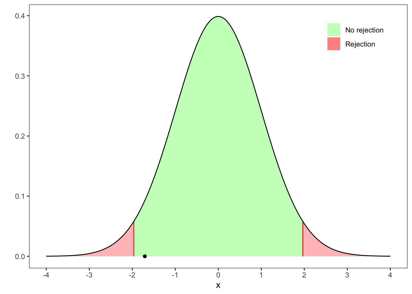
For example, let’s simulate a sample $X_n$ of $n=500$ observations from a normal distribution (i.e. $X_n\sim \mathcal{N}(2,4^2)$) and consider the following sets of hypothesis, i.e. $${\mathcal{H}}_0:\mu (X)=2.4{\mathcal{H}}_1:\mu (X)\ne 2.4$$ The statistic test is defined as $$T(X_n)=\sqrt{500}\cdot \frac{\mu (X_n)-2.4}{\sigma (X_n)}\stackrel{{\mathcal{H}}_0}{\sim }t(499)\text{.}$$ Since it is a two-tailed test the critical value for a significance level $\alpha$, denoted as $t_{\alpha }$, is such that: $$\begin{array}{rl}\alpha & =\mathbb{P}([T(X_n)<-t_{\alpha /2}]\cup [T(X_n)>t_{\alpha /2}])\\ \Updownarrow & \\ t_{\alpha /2}& ={\mathbb{P}}^{-1}(\mathbb{P}(T(X_n)>t_{\alpha /2}))\text{,}\end{array}$$ where ${\mathbb{P}}^{-1}$ and $\mathbb{P}$ are respectively the quantile and distribution functions of a Student-$t$. If the statistic test $|T(X_n)|>|t_{\alpha /2}|$, then we reject ${\mathcal{H}}_0$ and so the mean of the sample is significantly different from 2.4. More precisely, with $\alpha =0.05$, the critical value of a Student-t with 499 degrees of freedom is $t_{\alpha /2}=1.9604$.

# Statistic T
z <- sqrt(n)*(mean(x) - mu_0)/sd(x)
# Student-t density
pdf <- dt(x_grid, df = n-1)
# Critical value left 
z_left <- c(qt(alpha/2, df = n-1), dt(qt(alpha/2, df = n-1), df = n-1))
# Critical value right 
z_right <- c(qt(1-alpha/2, df = n-1), dt(qt(1-alpha/2, df = n-1), df = n-1))

# Area left tail 
x_left <- x_grid[x_grid < z_left[1]]
y_left <- dt(x_left, df = n-1)
# Area right tail 
x_right <- x_grid[x_grid > z_right[1]]
y_right <- dt(x_right, df = n-1)
# Central area
x_centre <- x_grid[x_grid > z_left[1] & x_grid < z_right[1]]
y_centre <- dt(x_centre, df = n-1)
ggplot()+
  geom_segment(aes(x = z_left[1], xend = z_left[1], y = 0, yend = z_left[2]), color = "red")+
  geom_segment(aes(x = z_right[1], xend = z_right[1], y = 0, yend = z_right[2]), color = "red")+
  geom_ribbon(aes(x = x_centre, ymin = 0, ymax = y_centre, fill = "norej"), alpha = 0.3)+
  geom_ribbon(aes(x = x_left, ymin = 0, ymax = y_left, fill = "rej"), alpha = 0.3)+
  geom_ribbon(aes(x = x_right, ymin = 0, ymax = y_right, fill = "rej"), alpha = 0.3)+
  geom_line(aes(x_grid, pdf))+
  geom_point(aes(z, 0), color = "black")+
  scale_fill_manual(values = c(rej = "red", norej = "green"), 
                    labels = c(rej = "Rejection", norej = "No rejection")) + 
  scale_x_continuous(breaks = x_breaks) +
  labs(y = "", x = "x", fill = NULL)+
  theme_bw()+
  theme(
    legend.position = c(.95, .95),
    legend.justification = c("right", "top"),
    legend.box.just = "right",
    legend.margin = margin(6, 6, 6, 6),
    panel.grid = element_blank())

Figure 23.1: Two-tailed test on the mean.

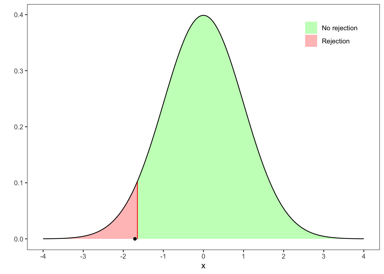
Let’s consider another kind of hypothesis, $${\mathcal{H}}_0:\mu (X)\ge 2.4{\mathcal{H}}_1:\mu (X)<2.4$$ The statistic test $T(X_n)$ do not changes, however the null hypothesis implies a left-tailed test. Hence, the critical value is $t_{\alpha }$ is such that $\mathbb{P}(x<t_{\alpha })=0.05$. Applying the quantile function ${\mathbb{P}}^{-1}$ of a student-$t$ we obtain: $$\begin{array}{rl}\alpha & =\mathbb{P}(T(X_n)<t_{\alpha })\\ \Updownarrow & \\ t_{\alpha }& ={\mathbb{P}}^{-1}(\mathbb{P}(T(X_n)<t_{\alpha }))\text{,}\end{array}$$ where ${\mathbb{P}}^{-1}$ and $\mathbb{P}$ are respectively the quantile and distribution functions of a Student-$t$. In this case, with $\alpha =0.05$, the critical value of a Student-t with 499 degrees of freedom is $t_{\alpha /2}=-1.6451$. Therefore, if $T(X_n)<-1.6451$ we do not reject the null hypothesis, i.e. $\mu (X_n)$ is greater than ${\mu }_0$, otherwise we reject it and $\mu (X_n)$ is lower than ${\mu }_0$.

# Critical value left 
z_left <- c(qt(alpha, df = n-1), dt(qt(alpha, df = n-1), df = n-1))
# Area left tail 
x_left <- x_grid[x_grid < z_left[1]]
y_left <- dt(x_left, df = n-1)
# Area right tail 
x_right <- x_grid[x_grid > z_left[1]]
y_right <- dt(x_right, df = n-1)
ggplot()+
  geom_segment(aes(x = z_left[1], xend = z_left[1], y = 0, yend = z_left[2]), color = "red")+
  geom_ribbon(aes(x = x_left, ymin = 0, ymax = y_left, fill = "rej"), alpha = 0.3)+
  geom_ribbon(aes(x = x_right, ymin = 0, ymax = y_right, fill = "norej"), alpha = 0.3)+
  geom_line(aes(x_grid, pdf))+
  geom_point(aes(z, 0), color = "black")+
  scale_fill_manual(values = c(rej = "red", norej = "green"), 
                    labels = c(rej = "Rejection", norej = "No rejection")) + 
  scale_x_continuous(breaks = x_breaks) +
  labs(y = "", x = "x", fill = NULL)+
  theme_bw()+
  theme_bw()+
  theme(
    legend.position = c(.95, .95),
    legend.justification = c("right", "top"),
    legend.box.just = "right",
    legend.margin = margin(6, 6, 6, 6),
    panel.grid = element_blank())

Figure 23.2: Left-tailed test on the mean.

In this case we reject the null hypothesis, hence $\mu (X_n)$ is lower than ${\mu }_0$.

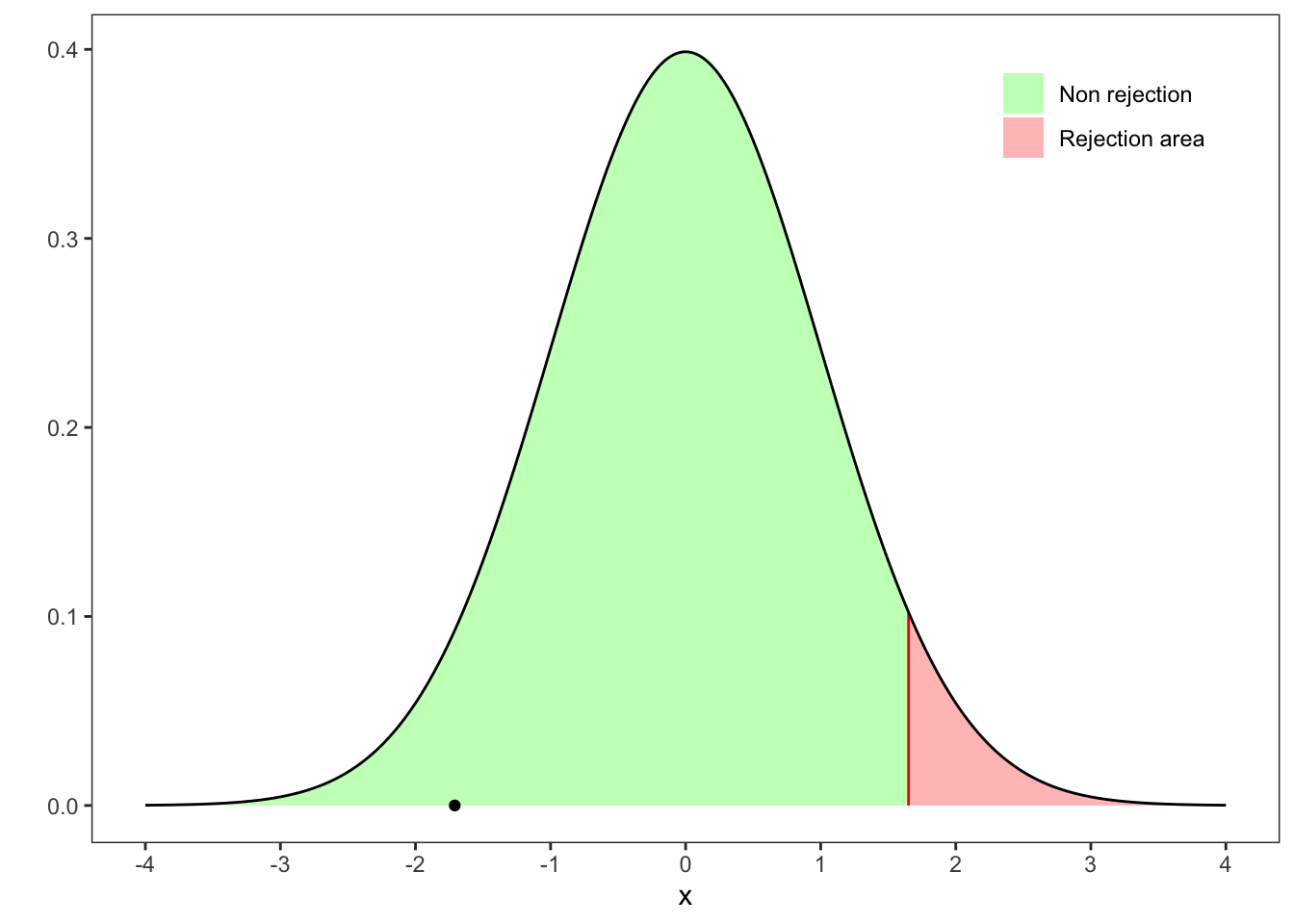
Lastly, let’s consider the right-tailed case, i.e. $$H_0:\mu (X)\le 2.4H_1:\mu (X)>2.4$$ It is always one-side test, but in this case is right-tailed. Hence, the critical value $t_{\alpha }$ is such that $$\begin{array}{rl}1-& \alpha =\mathbb{P}(T(X_n)<t_{\alpha })\\ \Updownarrow & \\ t_{\alpha }& ={\mathbb{P}}^{-1}(\mathbb{P}(T(X_n)<t_{\alpha }))\text{,}\end{array}$$ where ${\mathbb{P}}^{-1}$ and $\mathbb{P}$ are respectively the quantile and distribution functions of a Student-$t$. In this case, with $\alpha =0.05$, the critical value of a Student-t with 499 degrees of freedom is $t_{\alpha /2}=1.6451$. Therefore, if $T(X_n)<1.6451$ we do not reject the null hypothesis, i.e. $\mu (X_n)$ is lower than ${\mu }_0$, otherwise we reject it and $\mu (X_n)$ is greater than ${\mu }_0$. Coherently with the previous test performed in Figure 23.2, a right railed test is not rejected in Figure 23.3, hence $\mu (X_n)$ is lower than ${\mu }_0=2.4$.

# Critical value right 
z_right <- c(qt(1-alpha, df = n-1), dt(qt(1-alpha, df = n-1), df = n-1))
# Area right tail 
x_left <- x_grid[x_grid > z_right[1]]
y_left <- dt(x_left, df = n-1)
# Area right tail 
x_right <- x_grid[x_grid < z_right[1]]
y_right <- dt(x_right, df = n-1)
ggplot()+
  geom_segment(aes(x = x_left[1], xend = x_left[1], y = 0, yend = z_right[2]), color = "red")+
  geom_ribbon(aes(x = x_left, ymin = 0, ymax = y_left, fill = "rej"), alpha = 0.3)+
  geom_ribbon(aes(x = x_right, ymin = 0, ymax = y_right, fill = "norej"), alpha = 0.3)+
  geom_line(aes(x_grid, pdf))+
  geom_point(aes(z, 0), color = "black")+
  scale_fill_manual(values = c(rej = "red", norej = "green"), 
                    labels = c(rej = "Rejection area", norej = "Non rejection")) + 
  scale_x_continuous(breaks = x_breaks) +
  labs(y = "", x = "x", fill = NULL)+
  theme_bw()+
  theme(
    legend.position = c(.95, .95),
    legend.justification = c("right", "top"),
    legend.box.just = "right",
    legend.margin = margin(6, 6, 6, 6),
    panel.grid = element_blank())

Figure 23.3: Right-tailed test on the mean.

23.2 Tests for the means

Proposition 23.1 Let’s consider the $t$-test for the mean of a sample of identically and normally distributed random variables $X_n=(x_1,\dots ,x_i,\dots ,x_n)$. Then the test statistic $T(X_n)$ under ${\mathcal{H}}_0:\hat{\mu }(X_n)={\mu }_0$ is student-t distributed with $n-1$ degrees of freedom., i.e.  $$T(X_n)=\frac{\hat{\mu }(X_n)-{\mu }_0}{\frac{\hat{s}(X_n)}{\sqrt{n}}}\stackrel{{\mathcal{H}}_0}{\sim }{t}_{n-1}\text{,}$$ where $\hat{\mu }(X_n)$ is the sample mean $\hat{\mu }(X_n)$ and $\hat{\sigma }(X_n)$ the corrected sample variance. Moreover, for $n\to \mathrm{\infty }$: $$T(X_n)\stackrel{{\mathcal{H}}_0}{\underset{n\to \mathrm{\infty }}{⟶}}\mathcal{N}(0,1)\text{.}$$

Proof: Proposition 23.1

Proof. In the sample is normally distributed, the sample mean is also normally distributed, i.e.  $$M=\sqrt{n}\frac{\hat{\mu }(X_n)-{\mu }_0}{\sigma }\sim \mathcal{N}(0,1)\text{.}$$ Under normality the sample variance, that is a sum of the square of independent and normally distributed random variables, follows a ${\chi }^2$ distribution with $n-1$ degrees of freedom, i.e.  $$V=\frac{(n-1){\hat{s}}^2(X_n)}{{\sigma }^2}\sim {\chi }_{n-1}^2\text{.}$$ Notably, the ratio of a standard normal and a ${\chi }^2$ random variables (each one divided by the respective degrees of freedom) is exactly the definition of a Student-t random variable as in Equation 33.2. Hence, the ratio between the statistics $M$ and $V$ divided by their degrees of freedom reads $$\frac{M}{\sqrt{\frac{V}{n-1}}}=\sqrt{n}\frac{\hat{\mu }(X_n)-{\mu }_0}{\sigma }\sqrt{\frac{{\sigma }^2}{{\hat{s}}^2(X_n)}}=\sqrt{n}\frac{\hat{\mu }(X_n)-{\mu }_0}{{\hat{s}}^2(X_n)}\sim t_{n-1}\text{.}$$ The statistic test under $H_0$ follows a Student-t distribution with $n-1$ degrees of freedom. Notably, for large IID samples the statistic converges to a normal random variable independently from the distribution of $X$.

23.2.1 Test for two means and equal variances

Let’s consider two independent Gaussian populations with equal variance, i.e.  $$X_1\sim \mathcal{N}({\mu }_1,{\sigma }^2),X_2\sim \mathcal{N}({\mu }_2,{\sigma }^2)$$ Then, let’s consider two samples of unequal size, $n_1$ and $n_2$, with unknown means ${\mu }_1$ and ${\mu }_2$ and an equal unknown variance ${\sigma }^2$. Then, given the null hypothesis $$H_0={\mu }_1-{\mu }_2={\mu }_{\mathrm{\Delta }}\text{,}$$ the test statistic $$T(X_{n_1},X_{n_2})=\frac{\mu (X_{n_1})-\mu (X_{n_2})-{\mu }_{\mathrm{\Delta }}}{s_p\cdot \sqrt{\frac{1}{n_1}+\frac{1}{n_2}}}\sim t_{n_1+n_2-2}\text{,}$$ is Student-t distributed with $n_1+n_2-2$ degrees of freedom and $$s_p=\sqrt{\frac{(n_1-1){\hat{s}}^2(X_{n_1})+(n_2-1){\hat{s}}^2(X_{n_2})}{n_1+n_2-2}}\text{,}$$ where ${\hat{s}}^2(X_{n_1})$ and ${\hat{s}}^2(X_{n_2})$ are the sample corrected variances (Equation 9.11) of the two samples.

23.2.2 Test for two means and unequal variances

Let’s consider two independent Gaussian populations with different variance, i.e.  $$X_1\sim \mathcal{N}({\mu }_1,{\sigma }_1^2),X_2\sim \mathcal{N}({\mu }_2,{\sigma }_2^2)\text{.}$$ Then, let’s consider two samples of unequal size, $n_1$ and $n_2$, with unknown means ${\mu }_1$ and ${\mu }_2$ and an unequal unknown variance ${\sigma }^2$. Then, given the null hypothesis $$H_0={\mu }_1-{\mu }_2={\mu }_{\mathrm{\Delta }}\text{,}$$ Welch (1938) - Welch (1947) proposes a test statistic $$T(X_{n_1},X_{n_2})=\frac{\mu (X_{n_1})-\mu (X_{n_2})}{\sqrt{\frac{{\hat{s}}^2(X_{n_1})}{n_1}+\frac{{\hat{s}}^2(X_{n_2})}{n_2}}}\approx t_{\nu }\text{,}$$ that follows approximately a Student t-distribution under the null hypothesis, but with fractional degrees of freedom computed using the Welch–Satterthwaite approximation. This is a weighted average of the degrees of freedom from each group, reflecting the uncertainty due to unequal variances, i.e.  $$\nu =\frac{{(\frac{{\hat{s}}^2(X_{n_1})}{n_1}+\frac{{\hat{s}}^2(X_{n_1})}{n_2})}^2}{\frac{({\hat{s}}^2(X_{n_1}){)}^2}{n_1^2(n_1-1)}+\frac{({\hat{s}}^2(X_{n_1}){)}^2}{n_2^2(n_2-1)}}\text{.}$$ where $\nu$ is not necessary an integer.

23.3 Tests for the variances

23.3.1 F-test for two variances

Consider two independent normal samples, i.e.  $$X_{n_1}\sim \mathcal{N}({\mu }_1,{\sigma }_1^2),X_{n_2}\sim \mathcal{N}({\mu }_2,{\sigma }_2^2)\text{,}$$ where $n_1$ and $n_2$ are the number of observations in each sample. $$H_0:{\sigma }_1^2={\sigma }_2^2={\sigma }^2\text{.}$$ Knowing that the sample variance is chi2 distributed (Equation 9.15) let’s define the variables: $$T_1=(n_1-1)\frac{{\hat{s}}_1^2}{{\sigma }_1^2}\sim {\chi }_{n_1-1}^2,T_2=(n_2-1)\frac{{\hat{s}}_2^2}{{\sigma }_2^2}\sim {\chi }_{n_2-1}^2\text{.}$$ Then, since the ration of two independent ${\chi }^2$ divided by their respective degrees of freedom is $F$-distributed (Equation 33.3) the statistic $F$ is defined as: $$T(X_{n_1},X_{n_2})=\frac{\frac{T_1}{n_1-1}}{\frac{T_2}{n_1-1}}=\frac{\frac{{\hat{s}}_1^2}{{\sigma }_1^2}}{\frac{{\hat{s}}_2^2}{{\sigma }_2^2}}=\frac{{\hat{s}}_1^2{\sigma }_2^2}{{\hat{s}}_2^2{\sigma }_1^2}\sim {\text{F}}_{n_1-1,n_2,-1}$$ Under $H_0$ the two variances are assumed to be equal, i.e. ${\sigma }_1^2={\sigma }_2^2={\sigma }^2$, thus the statistic simplifies in: $$T(X_{n_1},X_{n_2})\stackrel{H_0}{=}\frac{{\hat{s}}_1^2}{{\hat{s}}_2^2}\sim {\text{F}}_{n_1-1,n_2,-1}$$ This means that the null hypothesis of equal variances can be rejected when F is as extreme or more extreme than the critical value obtained from the $\text{F}$-distribution with degrees of freedom $n_1-1$ and $n_2-1$ using a significance level $\alpha$.

Welch, B. L. 1938. “The Significance of the Difference Between Two Means When the Population Variances Are Unequal.” Biometrika 29 (3/4): 350–62. https://doi.org/10.1093/biomet/29.3-4.350.

———. 1947. “The Generalization of "Student’s" Problem When Several Different Population Variances Are Involved.” Biometrika 34 (1-2): 28–35. https://doi.org/10.1093/biomet/34.1-2.28.