21 Conditional variance processes
A stochastic process for the conditional variance can be used to specify a model of the form \[ Y_t = \mathbb{E}\{Y_t \mid \mathcal{F}_{t-1}\} + \sqrt{\mathbb{V}\{Y_t \mid \mathcal{F}_{t-1}\}} \cdot u_t \text{,} \] where the conditional mean and variance can both be stochastic. In the following section, we will explore models with constant conditional mean, i.e. \[ \mathbb{E}\{Y_t \mid \mathcal{F}_{t-1}\} = \mu \text{,} \] however the above expression can be generalized using AR or ARMA processes.
21.1 ARCH(p) process
The autoregressive conditionally heteroskedastic process (ARCH) was introduced in 1982 by Robert Engle (Engle (1982)) to model the conditional variance of a time series. It is often an empirical fact in economics that larger values in a time series are associated with larger variance. Let’s define an ARCH process of order \(p\) as: \[ \begin{aligned} & {} Y_t = \mu + e_t \\ & e_t = \sigma_t u_t \\ & \sigma_t^2 = \omega + \sum_{i=1}^{p} \alpha_i e_{t-i}^2 \end{aligned} \tag{21.1}\] where \(u_t\) is a standardized martingale difference sequence, i.e. \(\mathbb{E}\{u_t \mid \mathcal{F}_{t-1}\}=0\) and \(\mathbb{E}\{u_t^2 \mid \mathcal{F}_{t-1}\}=1\).
21.1.1 Moments
Proposition 21.1 The conditional mean of an ARCH(p) process (Equation 21.1) is equal to \[ \mathbb{E}\{Y_t \mid \mathcal{F}_{t-1}\} = \mu \text{.} \]
Proposition 21.2 The one-step conditional variance of an ARCH(p) process (Equation 21.1) is known given the information at time \(t-1\). For a general forecast horizon \(h\ge 1\) it reads: \[ \mathbb{V}\{Y_{t+h} \mid \mathcal{F}_{t}\} = \mathbb{E}\{\sigma_{t+h}^2 \mid \mathcal{F}_{t}\} \text{.} \]
The long-term (unconditional) expectation of the ARCH(p) variance \(\sigma_t^2\) reads \[ \mathbb{E}\{\sigma_t^2\} = \frac{\omega}{1 - \sum_{i=1}^{p} \alpha_i} \text{.} \] where \(\omega > 0\). It is clear that, to ensure finite long-term variance, the following condition on the ARCH parameters must be satisfied for all \(i \in \{1, \dots, p\}\), i.e. \[ \sum_{i=1}^{p} \alpha_i < 1 \text{,} \quad \alpha_i \ge 0 \text{.} \]
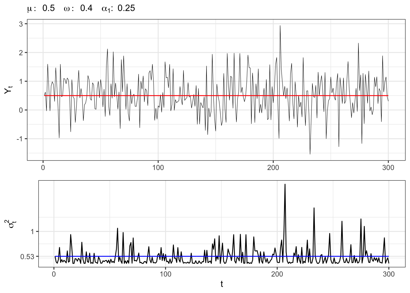
Example 21.1 Let’s simulate an ARCH(1) process with normal residuals, i.e. \[ \begin{aligned} & {} Y_t = \mu + e_t \\ & e_t = \sigma_t u_t \\ & \sigma_t^{2} = \omega + \alpha_1 e_{t-1}^2 \end{aligned} \] where \(u_t \sim \mathcal{N}(0,1)\).
ARCH(1) simulation
# Random seed
set.seed(1)
# *************************************************
#                      Inputs
# *************************************************
# Number of simulations
t_bar <- 300
# Long term mean of Yt
mu <- 0.5
# Intercept sigma2
omega <- 0.4
# ARCH parameters
alpha <- c(alpha1 = 0.25)
# *************************************************
#                    Simulation
# *************************************************
# Long-term variance
e_sigma2 <- omega / (1 - sum(alpha))
# Starting point
Yt <- rep(mu, 2)
# Initialization
sigma2_t <- rep(e_sigma2, 4)
# Simulate standardized residuals
u_t <- rnorm(t_bar, 0, 1)
# Initialize residuals
e_t <- sqrt(sigma2_t) * u_t
for(t in 2:t_bar){
  # ARCH components
  sum_arch <- alpha[1] * e_t[t-1]^2
  # Next-step variance
  sigma2_t[t] <- omega + sum_arch
  # Update simulated residuals
  e_t[t] <- sqrt(sigma2_t[t]) * u_t[t]
  # Update time series
  Yt[t] <- mu + e_t[t]
}
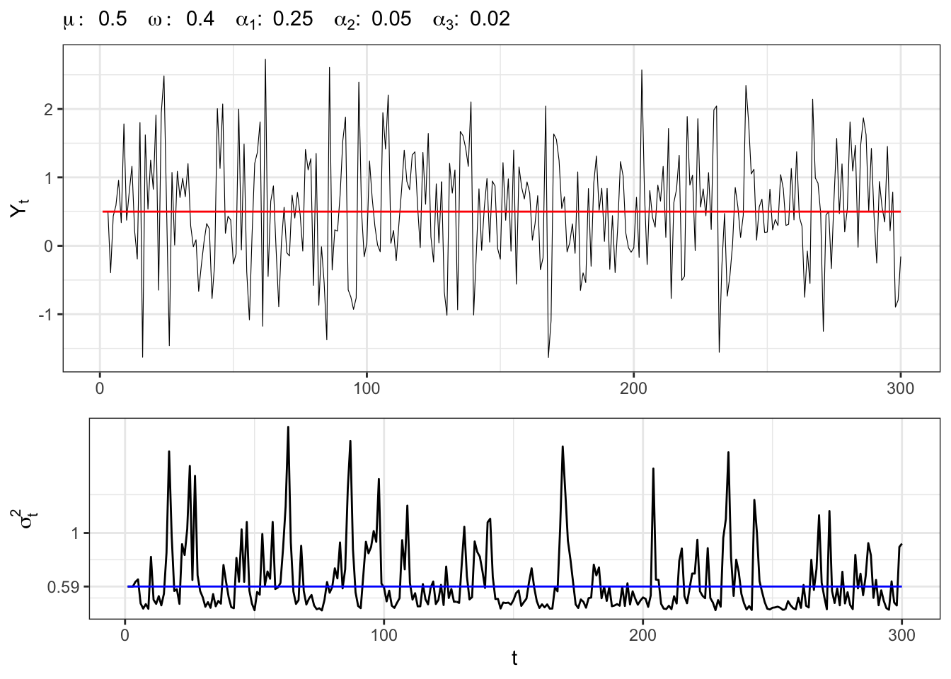
Example 21.2 Let’s simulate an ARCH(3) process with normal residuals, i.e. \[ \begin{aligned} & {} Y_t = \mu + e_t \\ & e_t = \sigma_t u_t \\ & \sigma_t^{2} = \omega + \alpha_1 e_{t-1}^2 + \alpha_2 e_{t-2}^2 + \alpha_3 e_{t-3}^2 \end{aligned} \] where \(u_t \sim \mathcal{N}(0,1)\).
ARCH(3) simulation
# Random seed
set.seed(2)
# *************************************************
#                      Inputs
# *************************************************
# Number of simulations
t_bar <- 300
# Long term mean of Yt
mu <- 0.5
# Intercept sigma2
omega <- 0.4
# ARCH parameters
alpha <- c(alpha1 = 0.25, alpha2 = 0.05, alpha3 = 0.02)
# *************************************************
#                    Simulation
# *************************************************
# Long-term variance
e_sigma2 <- omega / (1 - sum(alpha))
# Starting point
Yt <- rep(mu, 4)
# Initialization
sigma2_t <- rep(e_sigma2, 4)
# Simulate standardized residuals
u_t <- rnorm(t_bar, 0, 1)
# Initialize residuals
e_t <- sqrt(sigma2_t) * u_t
for(t in 4:t_bar){
  # ARCH components
  sum_arch <- alpha[1] * e_t[t-1]^2 + alpha[2] * e_t[t-2]^2 + alpha[3] * e_t[t-3]^2
  # Next-step variance
  sigma2_t[t] <- omega + sum_arch
  # Update simulated residuals
  e_t[t] <- sqrt(sigma2_t[t]) * u_t[t]
  # Update time series
  Yt[t] <- mu + e_t[t]
}
21.2 GARCH(p,q) process
As done with ARCH(p), with generalized autoregressive conditional heteroskedasticity (GARCH) we model the dependency of the conditional second moment. It represents a more parsimonious way to express the conditional variance. A GARCH(p,q) process is defined as: \[ \begin{aligned} & {} Y_t = \mu + e_t \\ & e_t = \sigma_t u_t \\ & \sigma_t^{2} = \omega + \sum_{i=1}^{p} \alpha_i e_{t-i}^2 + \sum_{j=1}^{q} \beta_j \sigma_{t-j}^2 \end{aligned} \] where \(u_t\) is a standardized martingale difference sequence, i.e. \(\mathbb{E}\{u_t \mid \mathcal{F}_{t-1}\}=0\) and \(\mathbb{E}\{u_t^2 \mid \mathcal{F}_{t-1}\}=1\).
Regarding the variance, the long-term expectation of \(\sigma_t^2\) reads \[ \mathbb{E}\{\sigma_t^2\} = \frac{\omega}{1 - \sum_{i=1}^{p} \alpha_i - \sum_{j=1}^{q} \beta_j} \text{,} \tag{21.2}\] where \(\omega > 0\). It is clear that, to ensure finite long-term variance, the following condition on the GARCH parameters must be satisfied: \[ \sum_{i=1}^{p} \alpha_i + \sum_{j=1}^{q} \beta_j < 1 \text{,} \] with \(\alpha_i \ge 0\) and \(\beta_j \ge 0\) for all \(i \in \{1, \dots, p\}\) and \(j \in \{1, \dots, q\}\).
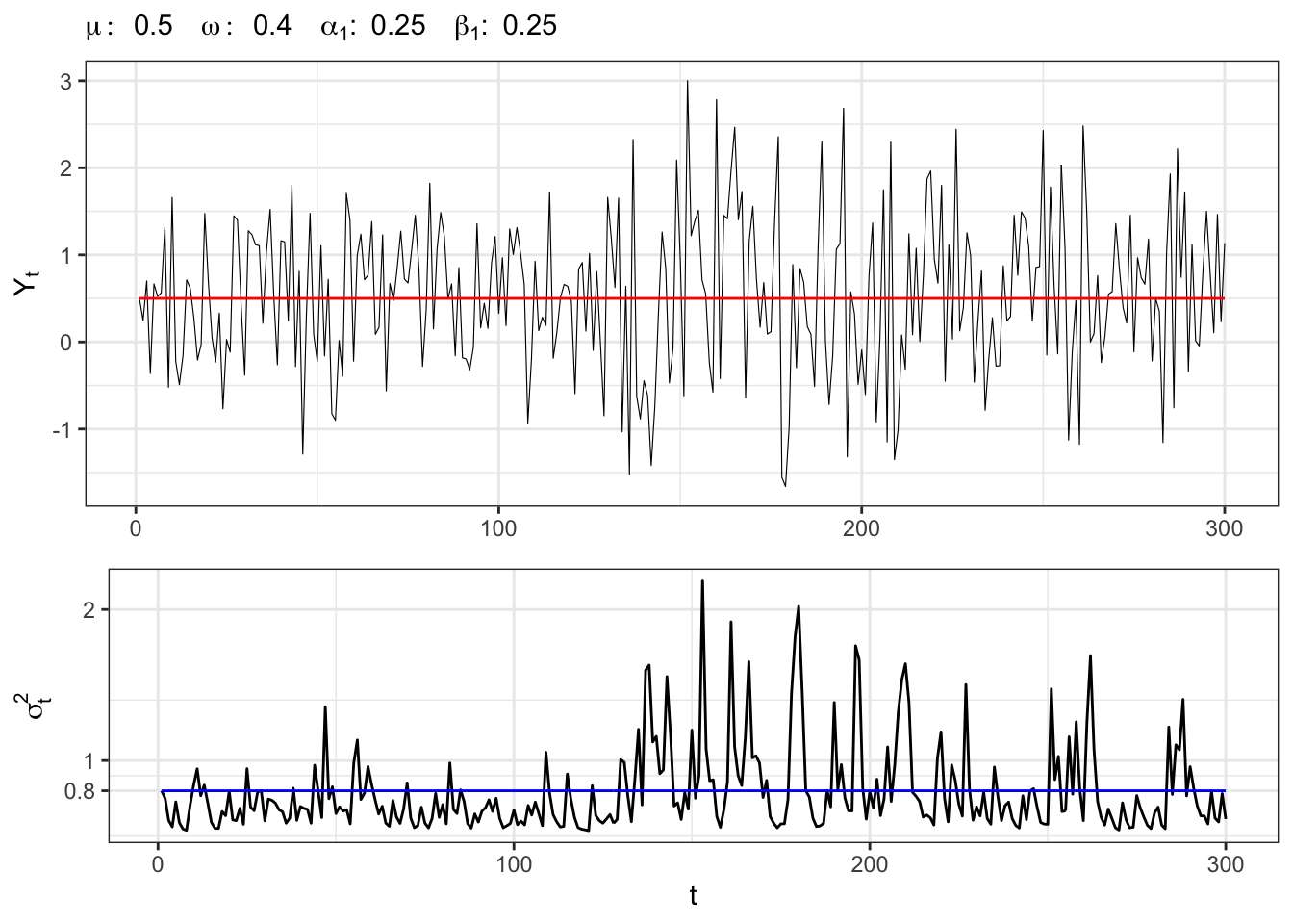
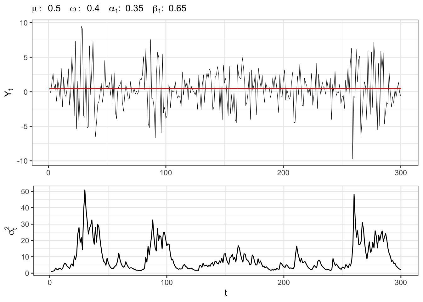
Example 21.3 Let’s simulate a GARCH(1,1) process with normal residuals, i.e. \[ \begin{aligned} & {} Y_t = \mu + e_t \\ & e_t = \sigma_t u_t \\ & \sigma_t^{2} = \omega + \alpha_1 e_{t-1}^2 + \beta_1 \sigma_{t-1}^2 \end{aligned} \] where \(u_t \sim \mathcal{N}(0,1)\).
GARCH(1,1) simulation
# Random seed
set.seed(3)
# *************************************************
#                      Inputs
# *************************************************
# Number of simulations
t_bar <- 300
# Long term mean of Yt
mu <- 0.5
# Intercept sigma2
omega <- 0.4
# ARCH parameters
alpha <- c(alpha1 = 0.25)
# GARCH parameters
beta <- c(beta1 = 0.25)
# *************************************************
#                    Simulation
# *************************************************
# Long-term variance
e_sigma2 <- omega / (1 - sum(alpha) - sum(beta))
# Starting point
Yt <- rep(mu, 2)
# Initialization
sigma2_t <- rep(e_sigma2, 4)
# Simulate standardized residuals
u_t <- rnorm(t_bar, 0, 1)
# Initialize residuals
e_t <- sqrt(sigma2_t) * u_t
for(t in 2:t_bar){
  # ARCH components
  sum_arch <- alpha[1] * e_t[t-1]^2
  # GARCH components
  sum_garch <- beta[1] * sigma2_t[t-1]
  # Next-step variance
  sigma2_t[t] <- omega + sum_arch + sum_garch
  # Update simulated residuals
  e_t[t] <- sqrt(sigma2_t[t]) * u_t[t]
  # Update time series
  Yt[t] <- mu + e_t[t]
}
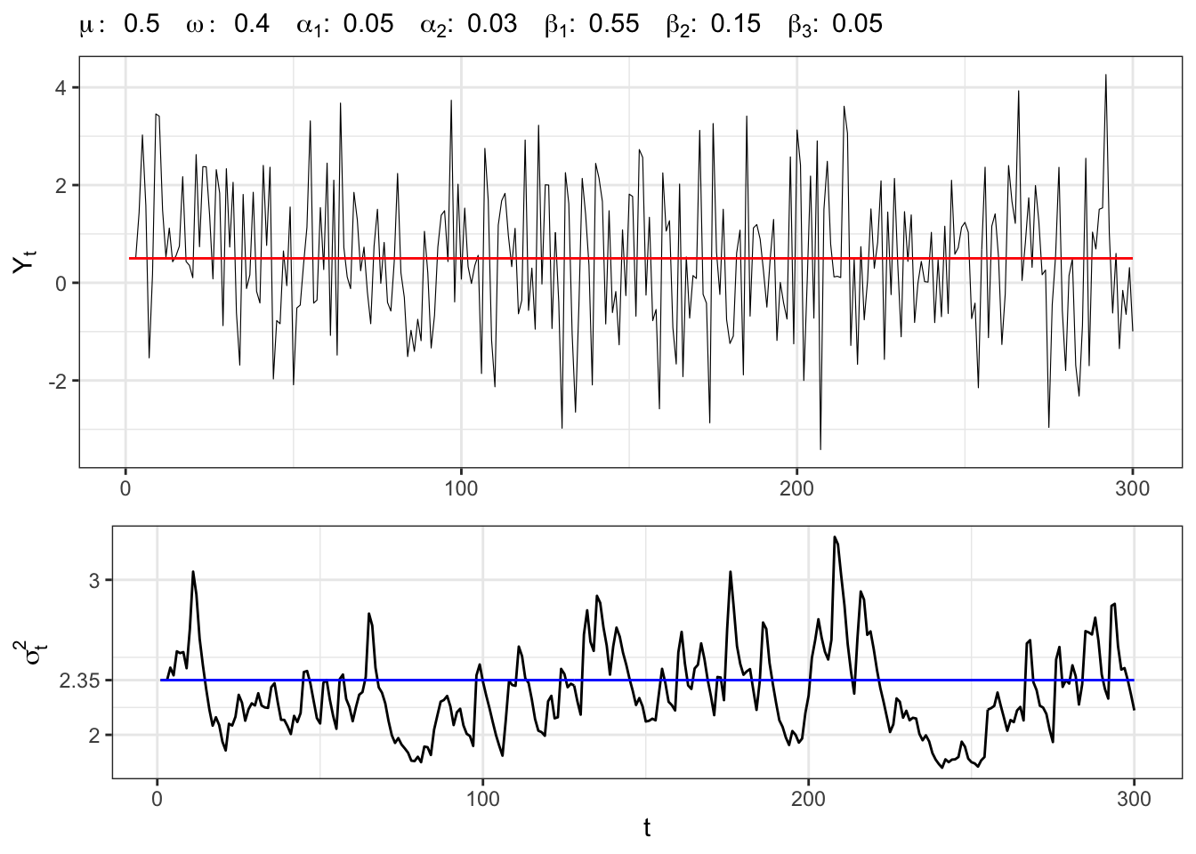
Example 21.4 Let’s simulate a GARCH(2,3) process with normal residuals, i.e. \[ \begin{aligned} & {} Y_t = \mu + e_t \\ & e_t = \sigma_t u_t \\ & \sigma_t^{2} = \omega + \alpha_1 e_{t-1}^2 + \alpha_2 e_{t-2}^2 + \beta_1 \sigma_{t-1}^2 + \beta_2 \sigma_{t-2}^2 + \beta_3 \sigma_{t-3}^2 \end{aligned} \] where \(u_t \sim \mathcal{N}(0,1)\).
GARCH(2,3) simulation
# Random seed
set.seed(4)
# *************************************************
#                      Inputs
# *************************************************
# Number of simulations
t_bar <- 300
# Long term mean of Yt
mu <- 0.5
# Intercept sigma2
omega <- 0.4
# ARCH parameters
alpha <- c(alpha1 = 0.05, alpha2 = 0.03)
# GARCH parameters
beta <- c(beta1 = 0.55, beta2 = 0.15, beta3 = 0.05)
# *************************************************
#                    Simulation
# *************************************************
# Long-term variance
e_sigma2 <- omega / (1 - sum(alpha) - sum(beta))
# Starting point
Yt <- rep(mu, 4)
# Initialization
sigma2_t <- rep(e_sigma2, 4)
# Simulate standardized residuals
u_t <- rnorm(t_bar, 0, 1)
# Initialize residuals
e_t <- sqrt(sigma2_t) * u_t
for(t in 4:t_bar){
  # ARCH components
  sum_arch <- alpha[1] * e_t[t-1]^2 + alpha[2] * e_t[t-2]^2
  # GARCH components
  sum_garch <- beta[1] * sigma2_t[t-1] + beta[2] * sigma2_t[t-2] + beta[3] * sigma2_t[t-3]
  # Next-step variance
  sigma2_t[t] <- omega + sum_arch + sum_garch
  # Update simulated residuals
  e_t[t] <- sqrt(sigma2_t[t]) * u_t[t]
  # Update time series
  Yt[t] <- mu + e_t[t]
}
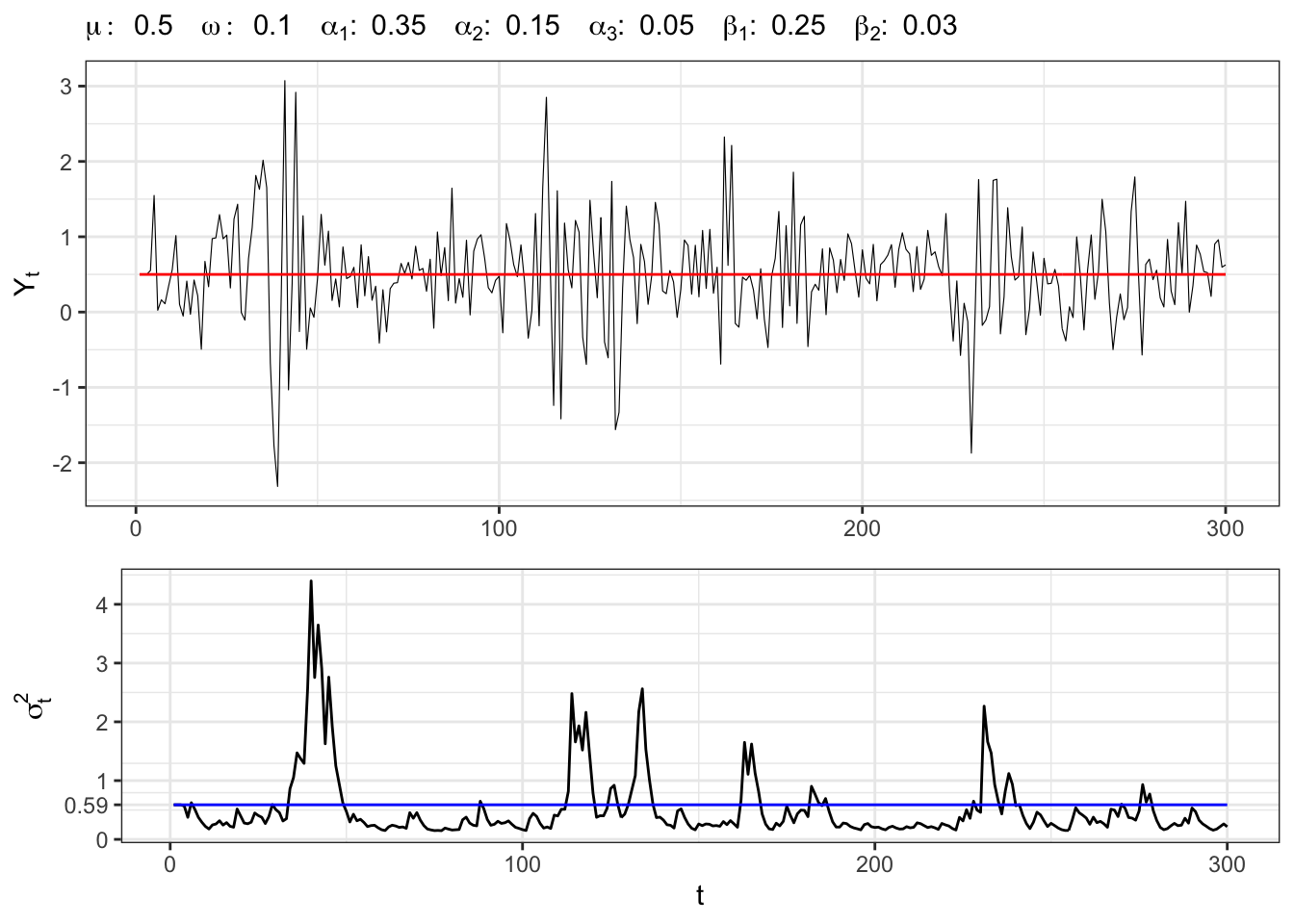
Example 21.5 Let’s simulate a GARCH(3,2) process with normal residuals, i.e. \[ \begin{aligned} & {} Y_t = \mu + e_t \\ & e_t = \sigma_t u_t \\ & \sigma_t^{2} = \omega + \alpha_1 e_{t-1}^2 + \alpha_2 e_{t-2}^2 + \alpha_3 e_{t-3}^2 + \beta_1 \sigma_{t-1}^2 + \beta_2 \sigma_{t-2}^2 \end{aligned} \] where \(u_t \sim \mathcal{N}(0,1)\).
GARCH(3,2) simulation
# Random seed
set.seed(5)
# *************************************************
#                      Inputs
# *************************************************
# Number of simulations
t_bar <- 300
# Long term mean of Yt
mu <- 0.5
# Intercept sigma2
omega <- 0.1
# ARCH parameters
alpha <- c(alpha1 = 0.35, alpha2 = 0.15, alpha3 = 0.05)
# GARCH parameters
beta <- c(beta1 = 0.25, beta2 = 0.03)
# *************************************************
#                    Simulation
# *************************************************
# Long-term variance
e_sigma2 <- omega / (1 - sum(alpha) - sum(beta))
# Starting point
Yt <- rep(mu, 4)
# Initialization
sigma2_t <- rep(e_sigma2, 4)
# Simulate standardized residuals
u_t <- rnorm(t_bar, 0, 1)
# Initialize residuals
e_t <- sqrt(sigma2_t) * u_t
for(t in 4:t_bar){
  # ARCH components
  sum_arch <- alpha[1] * e_t[t-1]^2 + alpha[2] * e_t[t-2]^2 + alpha[3] * e_t[t-3]^2
  # GARCH components
  sum_garch <- beta[1] * sigma2_t[t-1] + beta[2] * sigma2_t[t-2]
  # Next-step variance
  sigma2_t[t] <- omega + sum_arch + sum_garch
  # Update simulated residuals
  e_t[t] <- sqrt(sigma2_t[t]) * u_t[t]
  # Update time series
  Yt[t] <- mu + e_t[t]
}
21.3 IGARCH
Many variants of the standard GARCH process were developed in the literature. For example, the Integrated Generalized Autoregressive Conditional Heteroskedasticity (IGARCH(p,q)) is a restricted version of the GARCH, where the persistence parameters sum to one and imply a unit root in the GARCH variance recursion, with the condition \[ \sum_{i=1}^{p} \alpha_i + \sum_{j=1}^{q} \beta_j = 1 \text{.} \] In GARCH(p, q), the sum of coefficients being less than 1 ensures stationarity (finite unconditional variance) while in IGARCH(p, q), the sum is exactly 1, so the process is nonstationary in variance: the conditional variance has a persistent memory, and the shocks to volatility accumulate over time. The process is strictly stationary under some conditions (see Nelson (1990)), but it has infinite unconditional variance.
Example 21.6 Let’s simulate an iGARCH(1,1) process with normal residuals, i.e. \[ \begin{aligned} & {} Y_t = \mu + e_t \\ & e_t = \sigma_t u_t \\ & \sigma_t^{2} = \omega + \alpha_1 e_{t-1}^2 + (1 - \alpha_1) \sigma_{t-1}^2 \end{aligned} \] where \(u_t \sim \mathcal{N}(0,1)\).
iGARCH(1,1) simulation
# Random seed
set.seed(6)
# *************************************************
#                      Inputs
# *************************************************
# Number of simulations
t_bar <- 300
# Long term mean of Yt
mu <- 0.5
# Intercept sigma2
omega <- 0.4
# ARCH parameters
alpha <- c(alpha1 = 0.35)
# *************************************************
#                    Simulation
# *************************************************
# Starting point
Yt <- rep(mu, 2)
# Initialization
sigma2_t <- rep(1, 2)
# Simulate standardized residuals
u_t <- rnorm(t_bar, 0, 1)
# Initialize residuals
e_t <- sqrt(sigma2_t) * u_t
for(t in 2:t_bar){
  # ARCH components
  sum_arch <- alpha[1] * e_t[t-1]^2
  # GARCH components
  sum_garch <- (1 - alpha[1]) * sigma2_t[t-1]
  # Next-step variance
  sigma2_t[t] <- omega + sum_arch + sum_garch
  # Update simulated residuals
  e_t[t] <- sqrt(sigma2_t[t]) * u_t[t]
  # Update time series
  Yt[t] <- mu + e_t[t]
}
21.4 GARCH-M
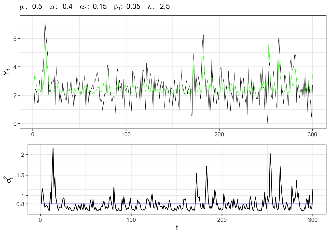
The GARCH in-mean (GARCH-M) model adds a stochastic term into the mean equation. This is motivated especially in financial theories (e.g., risk-return trade-off) suggesting that expected returns may depend on volatility, i.e. \[ \begin{aligned} & {} Y_t = \mu + \lambda \sigma_t^2 + e_t \\ & e_t = \sigma_t u_t \\ & \sigma_t^{2} \text{ follows a GARCH}(p,q) \text{ recursion} \end{aligned} \] The effect of the parameter \(\lambda\) is a shift of the mean of the process. If \(Y_t\) are, for example, financial returns, a \(\lambda > 0\) would imply that higher volatility increases expected return, consistent with risk-premium theories. Instead, when \(\lambda < 0\), it could reflect behavioral phenomena or model misspecification. The unconditional mean of \(Y_t\) becomes \[ \mathbb{E}\{Y_t\} = \mu + \lambda \mathbb{E}\{\sigma_t^2\} \text{,} \] while the conditional mean \[ \mathbb{E}\{Y_{t+h} \mid \mathcal{F}_t\} = \mu + \lambda \mathbb{E}\{\sigma^2_{t+h} \mid \mathcal{F}_t\} \text{.} \]
Example 21.7 Let’s simulate a GARCH-M(1,1) process with normal residuals, i.e. \[ \begin{aligned} & {} Y_t = \mu + \lambda \sigma^2_t + e_t \\ & e_t = \sigma_t u_t \\ & \sigma_t^{2} = \omega + \alpha_1 e_{t-1}^2 + \beta_1 \sigma_{t-1}^2 \end{aligned} \] where \(u_t \sim \mathcal{N}(0,1)\).
GARCH-M(1,1) simulation
# Random seed
set.seed(7)
# *************************************************
#                      Inputs
# *************************************************
# Number of simulations
t_bar <- 300
# Long term mean of Yt
mu <- 0.5
# Intercept sigma2
omega <- 0.4
# ARCH parameters
alpha <- c(alpha1 = 0.15)
# Mean param
lambda <- 2.5
# GARCH parameters
beta <- c(beta1 = 0.35)
# *************************************************
#                    Simulation
# *************************************************
# Long-term variance
e_sigma2 <- omega / (1 - sum(alpha) - sum(beta))
# Starting point
Yt <- rep(mu, 2)
# Initialization
sigma2_t <- rep(e_sigma2, 4)
# Simulate standardized residuals
u_t <- rnorm(t_bar, 0, 1)
# Initialize residuals
e_t <- sqrt(sigma2_t) * u_t
for(t in 2:t_bar){
  # ARCH components
  sum_arch <- alpha[1] * e_t[t-1]^2
  # GARCH components
  sum_garch <- beta[1] * sigma2_t[t-1]
  # Next-step variance
  sigma2_t[t] <- omega + sum_arch + sum_garch
  # Update simulated residuals
  e_t[t] <- sqrt(sigma2_t[t]) * u_t[t]
  # Update time series
  Yt[t] <- mu + sigma2_t[t] * lambda + e_t[t]
}