18  Time series

A stochastic process is a collection of random variables $\{X_t{\}}_{t\in \mathcal{T}}$ defined on a probability space $(\mathrm{\Omega },\mathcal{B},\mathbb{P})$ and assuming values in ${\mathbb{R}}^k$ with $k\ge 1$. The index set $\mathcal{T}$ is usually the half-like $[0,\mathrm{\infty })$, but can be also an interval $[a,b]$ or a subset of ${\mathbb{R}}^k$.

While a stochastic process has a crystal clear, mathematical definition. A time series is a less precise notion, and people use time series to refer to two related but different objects. A time series can be seen as a stochastic process indexed by integers or some regular, incremental unit of time that can in a sense by mapped to integers (eg. minutely, hourly, daily, monthly data). A time series can be understood as a collection of time-value–data-point pairs. while a stochastic process is the mathematical description of a distribution of time series. Some time series are a realization of stochastic processes or one can use a stochastic process as a model to generate a time series.

Definition 18.1 ($\mathbf{\text{Filtration}}$)
Let $(\mathrm{\Omega },\mathcal{B},\mathbb{P})$ be a probability space and let $\mathcal{T}$ be an index set. If for every $t\in \mathcal{T}$, one have that ${\mathcal{F}}_t$ is a sub-$\sigma$-algebra of $\mathcal{B}$ and for every $k\le t$ holds ${\mathcal{F}}_k\subseteq {\mathcal{F}}_t$, then the family of sub-$\sigma$-algebras denoted with $$\{{\mathcal{F}}_t{\}}_{t\in \mathcal{T}}\text{,}$$ is called a filtration.

For example, considering a stochastic process $\{X_n{\}}_{n\in \mathbb{N}}$ and consider the sequence of sub-$\sigma$-algebras generated by $X_1,X_2,\dots ,X_n$, then ${\mathcal{F}}_n$ is a $\sigma$-algebra and $\{{\mathcal{F}}_n{\}}_{n\in \mathbb{N}}$ is a filtration, also called natural filtration, with respect to $\{X_n{\}}_{n\in \mathbb{N}}$. Formally, ${\mathcal{F}}_n$ is the smallest $\sigma$-algebra containing all events observable up to the index $n$, i.e.  $$\begin{array}{rl}& {\mathcal{F}}_0=\sigma (X_0)\\ & {\mathcal{F}}_1={\mathcal{F}}_0\cup \sigma (X_1)=\sigma (X_0,X_1)\\ & {\mathcal{F}}_2={\mathcal{F}}_1\cup \sigma (X_2)=\sigma (X_0,X_1,X_2)\\ & ⋮\\ & {\mathcal{F}}_n={\mathcal{F}}_{n-1}\cup \sigma (X_{t-1})=\sigma (X_0,X_1,X_2,\dots ,X_n)\end{array}$$

18.1 Stationarity

Definition 18.2 ($\mathbf{\text{Strongly stationary}}$)
A stochastic process $\{X_t{\}}_{t\in \mathcal{T}}$ is said to be strongly stationary if and only if for all set of index $\{t_1,t_2,\dots ,t_n\}\in \mathcal{T}$ and for every $h\ne 0$ $$\mathbb{P}(X_{t_1},X_{t_2},\dots ,X_{t_n})=\mathbb{P}(X_{t_{1+h}},X_{t_{2+h}},\dots ,X_{t_{n+h}})\text{.}$$ meaning that the joint distribution of an arbitrary number of random variables $X_{t_1},X_{t_2},\dots ,X_{t_n}$ do not change shifting the process, upward or downward, by a step $h$.

Definition 18.3 ($\mathbf{\text{Weakly stationary}}$)
A stochastic process $\{X_t{\}}_{t\in \mathcal{T}}$ is said to be weakly stationary (or covariance stationary) if and only if

1. $\mathbb{E}\{X_t\}=\mu$ and $|\mu |<\mathrm{\infty }$ for every $t\in \mathcal{T}$;
2. $\mathbb{E}\{X_t^2\}<\mathrm{\infty }$ for every $t\in \mathcal{T}$;
3. $\mathbb{C}v\{X_t,X_{t+h}\}=\gamma (h)$ and $|\gamma (h)|<\mathrm{\infty }$ for every $t\in \mathcal{T}$ and $h\ne 0$.

Hence, the covariance $\gamma (h)$ of a weakly stationary process does not depend on time $t$, but only on the temporal lag $h$ between two observations.

Strong does not imply weakly and viceversa

In general if a process is strong stationary (Definition 18.2) does not implies that it is also weakly stationary. For example, an independent and identically distributed Cauchy process is strongly stationary, but since its expectation and variance are not finite the process is not weakly stationary.

18.2 Notable processes

Definition 18.4 ($\mathbf{\text{IID process}}$)
A time series, $\{X_t{\}}_{t\in \mathcal{T}}$ where each $X_t$ is independent from the others and all $X_t$ has the same distribution for all $t$ is called independent and identically distributed process (IID). Such kind of process, usually denoted as $X_t\sim \text{IID}(0,{\sigma }^2)$, is strongly stationary (Definition 18.2). Moreover, if the mean and variance are finite, the covariance is zero and the process is also weakly stationary (Definition 18.3), i.e.  $${\gamma }_t(h)=\mathbb{C}v\{X_t,X_{t+h}\}=\mathbb{E}\{X_t{X}_{t+h}\}=\mathbb{E}\{X_t\}\mathbb{E}\{X_{t+h}\}=0\text{.}$$

Definition 18.5 ($\mathbf{\text{White noise}}$)
A stochastic process ${X_t}_{t\in \mathcal{T}}$, commonly denoted as $$\begin{array}{}\text{(18.1)}& X_t\sim \text{WN}(0,{\sigma }^2)\text{.}\end{array}$$ is called White Noise if satisfies the following properties:

1. The expectation is equal to zero, i.e. $\mathbb{E}\{X_t\}=0$ for all $t\in \mathcal{T}$.
2. The variance is finite and constant for all $t\in \mathcal{T}$, i.e. $\mathbb{V}\{X_t\}={\sigma }^2<\mathrm{\infty }$.
3. The process is uncorrelated over time for all $t\ne k$, i.e. $\mathbb{C}v\{X_t,X_k\}=0$.

A White Noise process is weakly stationary (Definition 18.3). In fact, the autocovariance function of the process depends on the lag, but not on time, i.e. it is equal to the variance for $t=s$ and is zero otherwise. This process is more general than an IID process (Definition 18.4), since it does not requires the stochastic independence of the time series for all $t$.

18.2.1 Martingales

Definition 18.6 ($\mathbf{\text{Martingale}}$) Let’s consider a probability space $(\mathrm{\Omega },\mathcal{B},\mathbb{P})$ and stochastic process $\{M_t{\}}_{t\in \mathcal{T}}$. Then, given a filtration $\mathcal{F}$, namely $\{{\mathcal{F}}_t{\}}_{t\in \mathcal{T}}$, the stochastic process $M_t$ is a martingale with respect to the filtration $\{{\mathcal{F}}_t{\}}_{t\in \mathcal{T}}$ if

1. $M_t$ is adapted to ${\mathcal{F}}_t$ in the sense that $M_t$ in included in the information contained in ${\mathcal{F}}_t$, i.e. $M_t$ is ${\mathcal{F}}_t$-measurable.
2. For any $0\le k<t$ $$\begin{array}{}\text{(18.2)}& \mathbb{E}\{M_t\mid {\mathcal{F}}_k\}=M_k\text{.}\end{array}$$

Definition 18.7 ($\mathbf{\text{Martingale difference sequence}}$)
Let’s consider a probability space $(\mathrm{\Omega },\mathcal{B},\mathbb{P})$ and stochastic process $\{D_t{\}}_{t\in \mathcal{T}}$. Then, given a filtration $\mathcal{F}$, namely $\{{\mathcal{F}}_t{\}}_{t\in \mathcal{T}}$, the stochastic process $D_t$ is a martingale difference sequence (MDS) with respect to the filtration $\{{\mathcal{F}}_t{\}}_{t\in \mathcal{T}}$ if $D_t$ is ${\mathcal{F}}_t$-measurable and for any $0\le k<t$ $$\begin{array}{}\text{(18.3)}& \mathbb{E}\{D_t\mid {\mathcal{F}}_k\}=0\text{.}\end{array}$$ This implies that $D_t$ is a mean-zero process uncorrelated with any information contained ${\mathcal{F}}_{t-1}$. The definition can be extended to a case where the filtration ${\mathcal{F}}_{t-1}$ includes also other processes $X_t$. In this case, $D_t$ is said to be an MDS conditionally to $X_t$ if the same condition in Equation 18.3 holds.

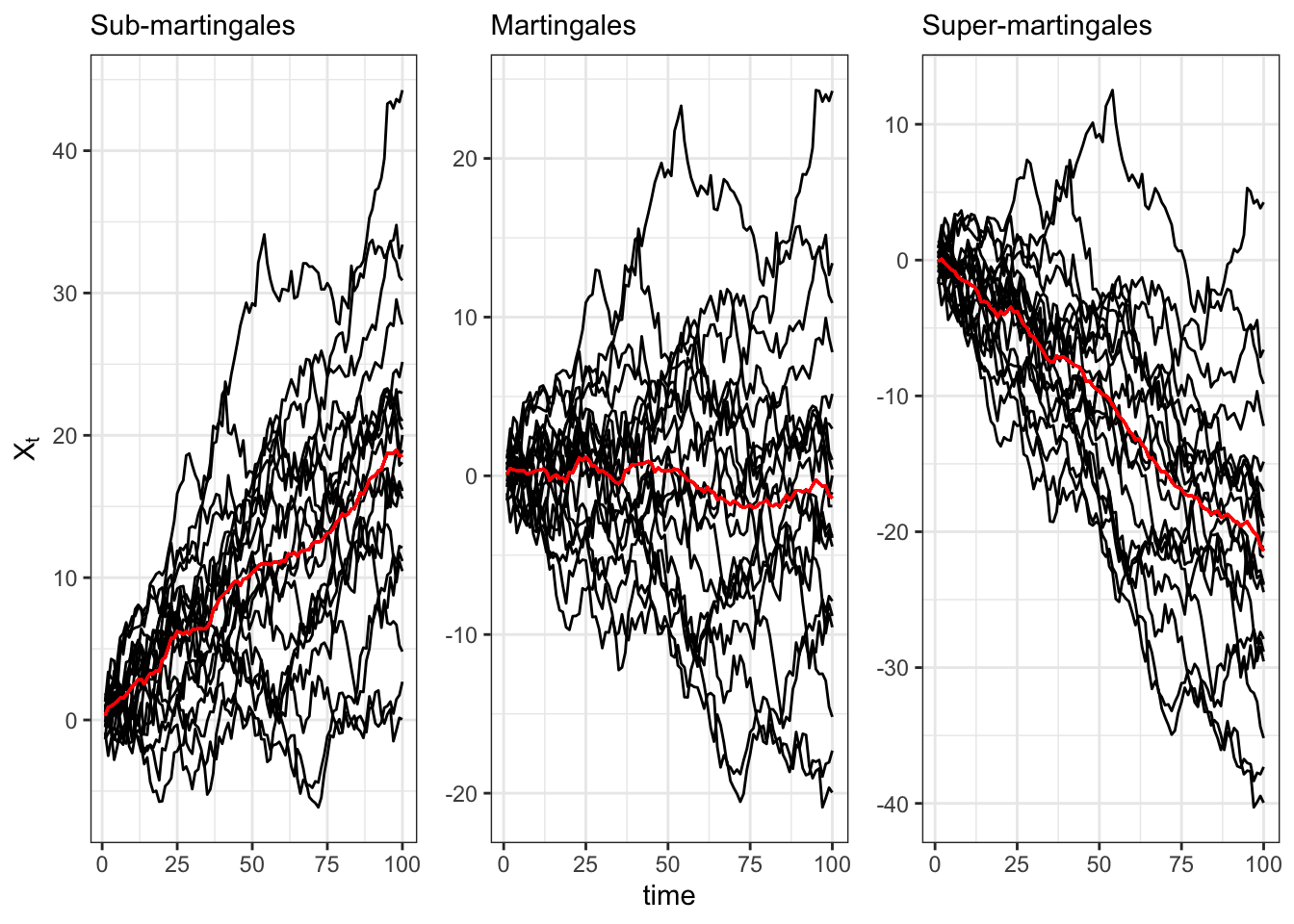
Super and sub-martingales

A stochastic process $\{X_t{\}}_{t\in \mathcal{T}}$ is said to be a sub-martingale if instead of Equation 18.2 we have that for any $0\le k<t$, $$\begin{array}{}\text{(18.4)}& \mathbb{E}\{X_t\mid {\mathcal{F}}_k\}\ge X_k\text{.}\end{array}$$ On the other hand it is said to be a super-martingale if $$\begin{array}{}\text{(18.5)}& \mathbb{E}\{X_t\mid {\mathcal{B}}_k\}\le X_k\text{.}\end{array}$$ From the above definitions it follows that to be a martingale (or an MDS) a stochastic process must be at the same time a super and sub-martingale.

set.seed(1)
# Number of observations
N <- 100
# Number of simulations
j_bar <- 20
# Predictable process
A_t <- rep(0.2, N)
X_sub <- X_mar <- X_sup <- list()
for(j in 1:j_bar){
  # Martingale 
  M_t <- rnorm(N, 0, 1)
  # Sub-martingale
  X_sub[[j]] <- dplyr::tibble(j = j, t = 1:N, X = cumsum(A_t + M_t))
  # Martingale 
  X_mar[[j]] <- dplyr::tibble(j = j, t = 1:N, X = cumsum(M_t))
  # Super-martingale 
  X_sup[[j]] <- dplyr::tibble(j = j, t = 1:N, X = cumsum(-A_t + M_t))
}

Figure 18.1: Simulation of a sub-martingale, martingale and super-martingale with expected value (red).

The concept of martingales is connected to the concept of predictability of a stochastic process.

Definition 18.8 ($\mathbf{\text{Predictable process}}$) Let’s consider a probability space $(\mathrm{\Omega },\mathcal{B},\mathbb{P})$ and stochastic process $\{A_t{\}}_{t\in \mathcal{T}}$. Then, let’s define a sequence of sub-$\sigma$ fields of $\mathcal{B}$, namely $\{{\mathcal{F}}_t{\}}_{t\in \mathcal{T}}$. Then, the stochastic process $A_t$ is predictable if

1. $A_0\in {\mathcal{F}}_0$;
2. For any $t\ge 0$ we have that $A_{t+1}\in {\mathcal{F}}_t$.

Then, we call the process predictable and increasing if $0=A_0\le A_1\le A_2\le \dots$.

Theorem 18.1 ($\mathbf{\text{Predictable process}}$) Any sub-martingale $\{X_t{\}}_{t\in \mathcal{T}}$, can be written in a unique way as the sum of a martingale $\{M_t{\}}_{t\in \mathcal{T}}$ and an increasing process $\{A_t{\}}_{t\in \mathcal{T}}$, i.e.  $$X_t=M_t+A_t\text{.}$$

18.3 Lag operator

The lag operator $L$ is a function that allows to translate a time series in time. In general, the lag operator associate at $y_t$ it’s lagged value $y_{t-1}$, i.e.  $$\begin{array}{}\text{(18.6)}& L(y_t)=y_{t-1}\text{.}\end{array}$$ More formally, $L$ is the operator that takes one whole time series and produces another; the second time series is the same as the first, but moved backwards or forward one point in time. From the definition, we list some properties related to the Lag operator, i.e. 

1. Backward $L^k(y_t)=y_{t-k}$.
2. Forward $L^{-k}(y_t=y_{t+k}$.
3. $L(a{y}_t+b{x}_t)=a{y}_{t-1}+b{x}_{t-1}$.

18.3.1 Polynomial of Lag operator

Given a time series $y_t$, it is possible to define polynomials of the Lag operator, i.e. $$\varphi (L)y_t=y_t+{\varphi }_1{y}_{t-1}+\cdots +{\varphi }_k{y}_{t-p}=\sum _{i=0}^p{\varphi }_i{y}_{t-i}\text{.}$$ where in general $$\begin{array}{}\text{(18.7)}& \varphi (L)=1+{\varphi }_{1}L+{\varphi }_2{L}^2+\cdots +{\varphi }_p{L}^p=\sum _{j=0}^p{\varphi }_j{L}^j\text{.}\end{array}$$

For the polynomial $\varphi (L)$ holds the factorization $$\varphi (L)=(1-\frac{1}{z_1}L)(1-\frac{1}{z_2}L)\dots (1-\frac{1}{z_k}L)=\prod _{i=1}^k(1-\frac{1}{z_i}L)\text{,}$$ where $z_1,\dots ,z_k$ are the complex solutions of the characteristic equation, i.e.  $$\varphi (z)=1+{\varphi }_{1}z+{\varphi }_2{z}^2+\cdots +{\varphi }_k{z}^k=0\text{.}$$ Hence the factorization holds true if and only if: $$|z_i|>1\mathrm{\forall }i⟺\frac{1}{|z_i|}<1\text{.}$$ In other words, the modulus of the solutions must outside the unit circle, otherwise the geometric series is not convergent and the factorization do not holds true anymore. The factorization of the lag polynomial allows us to define its inverse, i.e.  $${\varphi }^{-1}(L)=\prod _{i=1}^p{(1-\frac{1}{z_i}L)}^{-1}\text{,}$$ In fact, the inverse of the $i$-th term can be expressed with a Taylor expansion as infinite sum if and only if $|{\varphi }_i|<1$, i.e.  $${(1-{\varphi }_{i}L)}^{-1}=1+{\varphi }_{i}L+({\varphi }_{i}L{)}^2+\cdots =\sum _{j=0}^{\mathrm{\infty }}{\varphi }_i^j{L}^j⟺|{\varphi }_i|<1\text{.}$$ that is equivalent to $|z_i|>1$ for all $i$ since ${\varphi }_i=\frac{1}{z_i}$.

AR(1) and geometric series

For example, let’s consider an Autoregressive process of order 1, i.e. $$y_t={\varphi }_1{y}_{t-1}+e_t⟺\varphi (L)y_t=e_t⟺y_t={\varphi }^{-1}(L)e_t$$ In fact, $$\begin{array}{rl}\varphi (L)y_t& =y_t-{\varphi }_1{y}_{t-1}=\\ & =y_t-{\varphi }_1{y}_{t}L=\\ & =y_t(1-{\varphi }_{1}L)\end{array}$$ Considering such polynomial, its inverse polynomial $\varphi (L{)}^{-1}$, defined such that $\varphi (L){\varphi }^{-1}(L)=1$, is defined as geometric series, i.e.  $${\varphi }^{-1}(L)=1+{\varphi }_{1}L+({\varphi }_{1}L{)}^2+\cdots =\sum _{j=0}^{\mathrm{\infty }}{\varphi }_1^j{L}^j=\frac{1}{1-{\varphi }_{1}L}⟺|{\varphi }_1|<1\text{,}$$ that converges if and only if $|{\varphi }_1|<1$. Moreover, if $|{\varphi }_1|<1$ it is possible to prove that ${\varphi }^{-1}(L)$ is indeed the inverse polynomial of $\varphi (L)$, in fact: $$\begin{array}{rl}\varphi (L){\varphi }^{-1}(L)& =(1-{\varphi }_{1}L)\cdot \sum _{j=0}^{\mathrm{\infty }}({\varphi }_{1}L{)}^j=\\ & =\sum _{j=0}^{\mathrm{\infty }}({\varphi }_{1}L{)}^j-{\varphi }_{1}L\sum _{j=0}^{\mathrm{\infty }}({\varphi }_{1}L{)}^j=\\ & =\sum _{j=0}^{\mathrm{\infty }}({\varphi }_{1}L{)}^j-\sum _{j=0}^{\mathrm{\infty }}({\varphi }_{1}L{)}^{j+1}=\\ & =\sum _{j=0}^{\mathrm{\infty }}({\varphi }_{1}L{)}^j-\sum _{j=0}^{\mathrm{\infty }}({\varphi }_{1}L{)}^j+1=1\end{array}$$ Therefore, the process $y_t$ can be equivalently expressed as: $$y_t={\varphi }^{-1}(L)e_t=\sum _{j=0}^{\mathrm{\infty }}{\varphi }_1^j{e}_{t-j}$$ 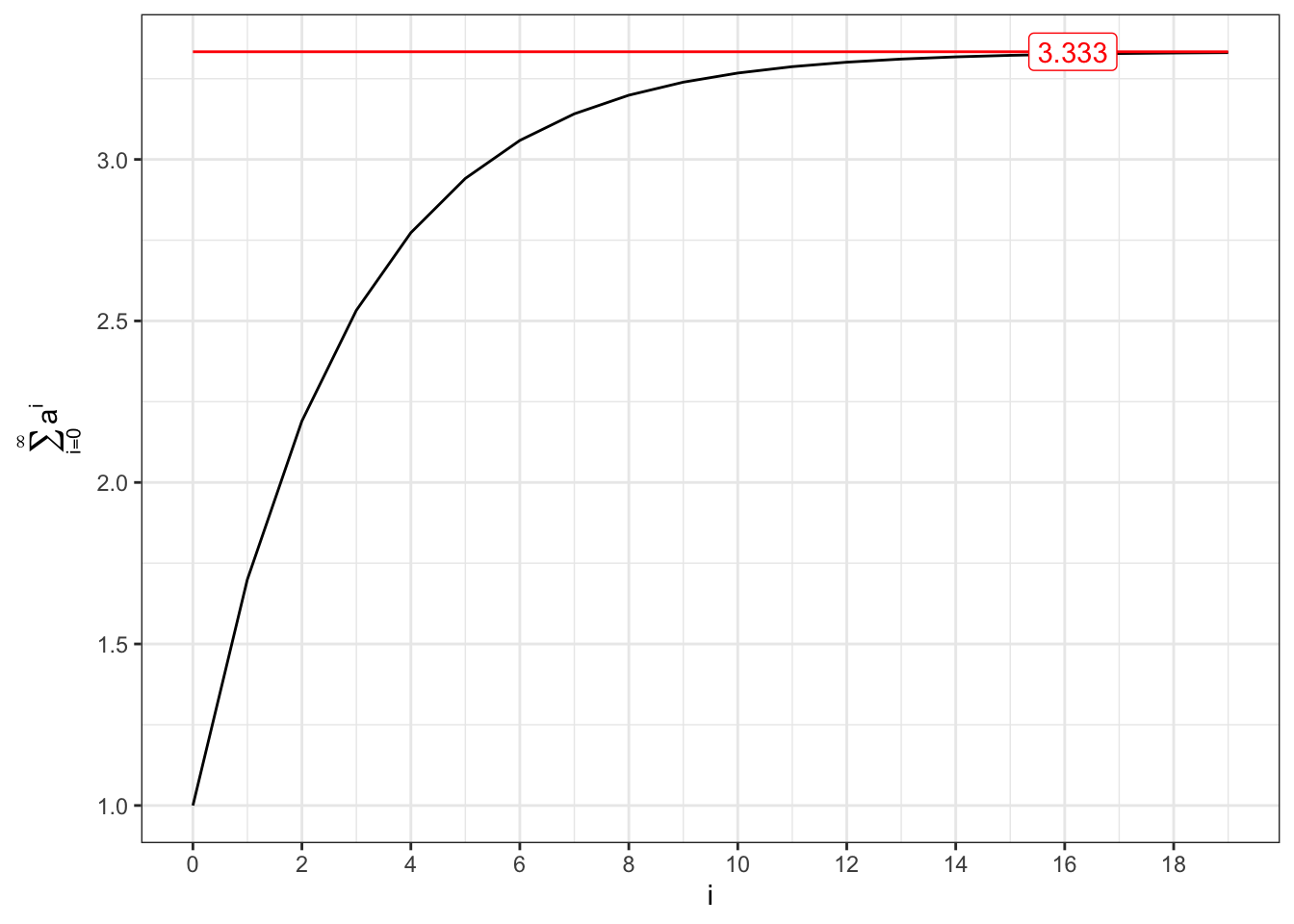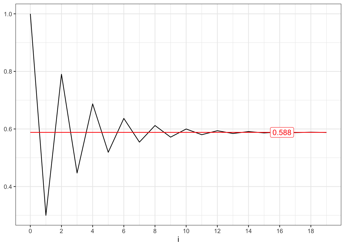The factorization of any polynomial of the form of $\varphi (L)$ is connected to the convergence of the following geometric series, i.e.  $$\sum _{j=0}^{\mathrm{\infty }}{\varphi }^j=\frac{1}{1-\varphi }⟺|\varphi |<1\text{.}$$

# *************************************************
#                      Inputs 
# *************************************************
a <- c(0.7, -0.7)
min_i <- 0
max_i <- 20
i <- seq(min_i, max_i - 1, 1)
y_breaks <- seq(min_i, max_i, 2)
x_labels <- quantile(i, 0.85)
# *************************************************
# Convergent series 0 < a < 1
series1 <- cumsum(a[1]^i)
limit1 <- 1/(1 - a[1])
# Convergent series -1 < a < 0
series2 <- cumsum(a[2]^i)
limit2 <- 1/(1 - a[2])

(a) $0<a<1$.

(b) $-1<a<0$.

Figure 18.2: Convergent series for AR(1) parameter (I).

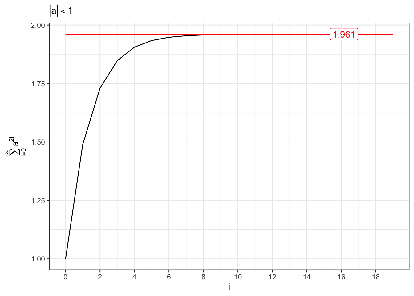
Another important series that is convergent only if and only if $|a|<1$, i.e.  $$\sum _{i=0}^{\mathrm{\infty }}{a}^{2i}=\frac{1}{1-a^2}⟺|a|<1\text{.}$$ Due to the square, in this case we do not distinguish between $0<a<1$ and $-1<a<0$ since they lead to the same result.

# Convergent series |a| < 1 
series1 <- cumsum(a[1]^(i*2))
limit1 <- 1/(1 - a[1]^2)

Figure 18.3: Convergent series for AR(1) parameter (II).