27  Bernoulli random variable

Figure 27.1: Distribution (left) and density (right) functions of a Bernoulli random variable.

27.1 Distribution and density
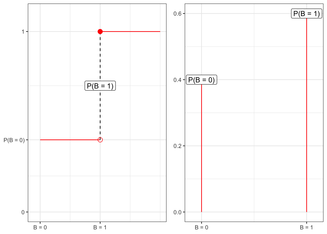
Definition 27.1 To construct a continuous distribution for a Bernoulli random variable, one can use the linear combination of two heavy side functions (Equation 1.10), i.e.  \[ F_B(x) = H(x) (1-p) + H(x-1) p \text{.} \tag{27.1}\] Given that the distribution function is specified in terms of Heavyside function, it is possible to take the derivative with respect to \(x\) to obtain the density function, i.e.  \[ f_B(x) = \delta(x) (1-p) + \delta(x-1) p \text{,} \tag{27.2}\] where \(\delta(x)\) is the Dirac function (Equation 1.11).

27.2 Characteristic function

Proposition 27.1 The characteristic function of a Bernoulli random variable reads explicitly: \[ \phi_B(t) = p e^{i t} + (1+p) \text{,} \tag{27.3}\] and similarly the moment generating function \[ \psi_{B}(t) = p e^{t} + (1+p) \text{.} \tag{27.4}\]

Proof. By the definition of characteristic function, one have to compute the following expectation, i.e.  \[ \begin{aligned} \phi_B(t) {} & = \mathbb{E}\{e^{it X}\} = \\ & = \int_{-\infty}^{\infty} e^{i t y} \left[p \delta(y -1) + (1-p) \delta(y)\right] dy = \\ & = p \int_{-\infty}^{\infty} e^{i t y} \delta(y -1) dy + \int_{-\infty}^{\infty} e^{i t y} \delta(y) dy - p \int_{-\infty}^{\infty} e^{i t y} \delta(y) dy = \\ & = p e^{i t \cdot 1} + e^{i t \cdot 0} - p e^{i t \cdot 0} = \\ & = p e^{i t} + (1 - p) \end{aligned} \] where, thanks to the fundamental property (Equation 1.12) of the Dirac delta the final expression simplifies.

27.3 Moments

Proposition 27.2 The \(n\)-th moment of a Bernoulli random variable with probability \(p\) reads \[ \mathbb{E}\{B^n\} = \mathbb{P}(B = 1) = p \text{,} \] for all \(n \in \mathbb{N}\).

Proof. Let’s considering the characteristic function of the Bernoulli (Equation 27.3) and take the derivative with respect to \(t\), i.e.  \[ \partial_t \phi_B(t) = i p e^{i t} \implies \mathbb{E}\{B\} = \frac{\partial_t \phi_B(t)}{i} = p e^{it} \text{.} \] Hence, the above expression evaluated in \(t = 0\) gives \[ \mathbb{E}\{B\} = \frac{\partial_t \phi_B(t)}{i^n} \biggl|_{t = 0} = p \text{.} \] Thanks to the exponential structure the \(n\)-th derivative reads \[ \partial_t^{n} \phi_B(t) = i^n p e^{i t} \implies \mathbb{E}\{B^n\} = \frac{\partial_t^{n} \phi_B(t)}{i^n} = p e^{it} \text{.} \] Therefore, all the \(n\) moments are exactly equal to \(p\). The same result is obtained with the moment generating function (Equation 27.4).