23 Stationarity tests
23.1 Dickey–Fuller test
The Dickey-Fuller test tests the null hypothesis that a unit root is present in an autoregressive (AR) model. The alternative hypothesis is different depending on which version of the test is used; it is usually “stationary” or “trend-stationary”. Let’s consider an AR(1) model, i.e. \[ X_t = \mu + \delta t + \phi X_{t-1} + u_t \text{,} \tag{23.1}\] or equivalently adding and subtracting \(X_{t-1}\) \[ \Delta X_t = \mu + \delta t + (\phi-1) X_{t-1} + u_t = \mu + \delta t + \gamma X_{t-1} + u_t, \qquad \gamma = \phi - 1 \text{,} \tag{23.2}\] where \(\Delta X_t = X_t - X_{t-1}\).
The set of hypotheses of the Dickey-Fuller test is: \[ \begin{aligned} & {} \mathcal{H}_0: \gamma = 0 \iff \phi=1 \iff (X_t \text{ is non-stationary}) \\ & \mathcal{H}_1: \gamma < 0 \iff \phi < 1 \iff (X_t \text{ is stationary}) \end{aligned} \] The Dickey–Fuller statistic is computed as \[ \text{DF} = \frac{\hat{\gamma}}{\mathbb{S}d\{\hat{\gamma}\}} \text{.} \] where \(\hat{\gamma}\) is the estimated parameter from the regression in Equation 23.2 and \(\mathbb{S}d\{\hat{\gamma}\}\) its standard error. However, the statistic does not follow the usual Student-t distribution under the unit-root null, so Dickey-Fuller critical values must be used.
23.2 Augmented Dickey–Fuller test
The augmented Dickey-Fuller test is a more general version of the Dickey-Fuller test for a general AR(p) model, i.e. \[ \Delta X_t = \mu + \delta t + \phi X_{t-1} + \sum_{i = 1}^{p} \phi_i \Delta X_{t-i} + u_t \text{.} \tag{23.3}\] The set of hypotheses of the augmented Dickey-Fuller test is: \[ \begin{aligned} & {} \mathcal{H}_0: \phi = 0 \iff (X_t \text{ is non-stationary}) \\ & \mathcal{H}_1: \phi < 0 \iff (X_t \text{ is stationary}) \end{aligned} \] The augmented Dickey–Fuller statistic (ADF) is computed as: \[ \text{ADF} = \frac{\hat{\phi}}{\mathbb{S}d\{\hat{\phi}\}} \text{.} \] where \(\hat{\phi}\) is the estimated parameter from the regression in Equation 23.3 and \(\mathbb{S}d\{\hat{\phi}\}\) its standard error. As in the Dickey-Fuller test, the critical values are computed using a specific table.
23.3 Kolmogorov-Smirnov test
The Kolmogorov-Smirnov two-sample test (KS) can be used to test whether two samples came from the same distribution. Let’s define the empirical distribution function \(F_{n}\) of \(n\) independent and identically distributed ordered observations \(x_{(i)}\) as \[ \hat{F}_{\mathbf{x}_n}(x) = \frac{1}{n}\sum_{i = 1}^{n} \mathbb{1}_{(-\infty, x]}(x_{(i)}) \text{.} \tag{23.4}\] The KS statistic quantifies a distance between the empirical distribution functions of two samples. The distribution of the KS statistic under the null hypothesis assumes that the samples are drawn from the same distribution, i.e. \[ \begin{aligned} & {} \mathcal{H}_0: X_t \text{ is stationary} \\ & \mathcal{H}_1: X_t \text{ is not stationary} \end{aligned} \] The test statistic for two samples with dimension \(n_1\) and \(n_2\) is defined as: \[ \text{KS}(\mathbf{x}_{n_1}, \mathbf{x}_{n_2}) = \underset{\forall x}{\sup}|F_{\mathbf{x}_{n_1}}(x) - F_{\mathbf{x}_{n_2}}(x)| \text{,} \] and for large samples \(\mathcal{H}_0\) is rejected at significance level \(\alpha\) if: \[ \text{KS}(\mathbf{x}_{n_1}, \mathbf{x}_{n_2}) > \sqrt{-\frac{1}{2} \ln\left(\frac{\alpha}{2}\right) \left(\frac{n_1+n_2}{n_1n_2}\right)} \text{.} \] Hence, since the statistic is always greater than or equal to zero, for a given statistic \(\text{KS}_{n_1, n_2}\) the large-sample tail approximation reads: \[ \mathbb{P}(X > \text{KS}(\mathbf{x}_{n_1}, \mathbf{x}_{n_2})) = \exp\left(-2 \frac{n_1n_2}{n_1+n_2} \text{KS}(\mathbf{x}_{n_1}, \mathbf{x}_{n_2})^2 \right) \text{.} \]
Example 23.1 Let’s consider 500 simulated observations of the random variable \(X\) drawn from a population distributed as \(X \sim N(0.4, 1)\). Then, considering it as a time series, let’s sample a random index to split the series at a point. Finally, as shown in Table 23.1, the null hypothesis, i.e. the two samples come from the same distribution, is not rejected at the significance level \(\alpha = 5\%\).
KS-test on a stationary time series
# ================ Setups ================
set.seed(5) # random seed
ci <- 0.05  # significance level (alpha)
n <- 500    # number of simulations
x <- rnorm(n, 0.4, 1) # stationary series
# ========================================
# Random time for splitting
t_split <- sample(n, 1)
# Split the time series
x1 <- x[1:t_split]
x2 <- x[(t_split+1):n]
# Number of elements for each sub-series
n1 <- length(x1)
n2 <- length(x2)
# Grid of values for computing KS-statistic
x_min <- quantile(x, 0.015)
x_max <- quantile(x, 0.985)
grid <- seq(x_min, x_max, length.out = 200)
# Empirical cdfs
cdf_n1 <- ecdf(x1)
cdf_n2 <- ecdf(x2)
# KS-statistic
ks_stat <- max(abs(cdf_n1(grid) - cdf_n2(grid)))
# Rejection level with probability alpha
rejection_lev <- sqrt(-0.5*log(ci/2))*sqrt((n1+n2)/(n1*n2))
# P-value
p.value <- exp(-2 * (n1*n2)/(n1+n2) * ks_stat^2)
KS-test plot
y_breaks <- seq(0, 1, 0.2)
y_labels <- paste0(format(y_breaks*100, digits = 2), "%")
grid_max <- grid[which.max(abs(cdf_n1(grid) - cdf_n2(grid)))]
ggplot()+
  geom_ribbon(aes(grid, ymax = cdf_n1(grid), ymin = cdf_n2(grid)),
              alpha = 0.5, fill = "green") +
  geom_line(aes(grid, cdf_n1(grid)))+
  geom_line(aes(grid, cdf_n2(grid)), color = "red")+
  geom_segment(aes(x = grid_max, xend = grid_max, y = cdf_n1(grid_max), yend = cdf_n2(grid_max)),
               linetype = "solid", color = "#102d6e")+
  geom_point(aes(grid_max, cdf_n1(grid_max)), color = "#102d6e")+
  geom_point(aes(grid_max, cdf_n2(grid_max)), color = "#102d6e")+
  scale_y_continuous(breaks = y_breaks, labels = y_labels)+
  labs(x = "x", y = "cdf")+
  theme_bw()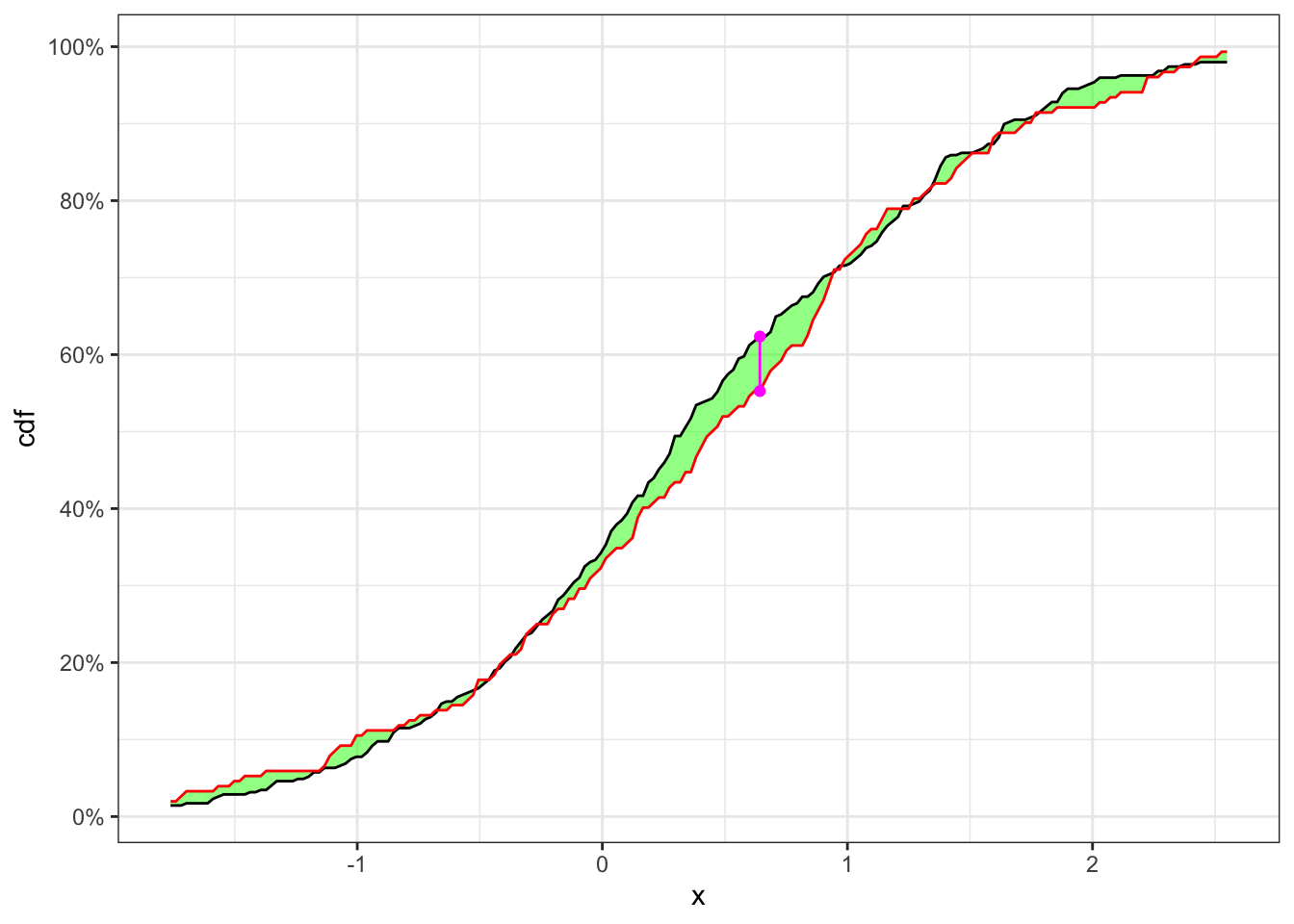
| \(\textbf{Index split}\) | \(\alpha\) | \(n_1\) | \(n_2\) | \(\text{KS}(\mathbf{x}_{n_1}, \mathbf{x}_{n_2})\) | p.value | \(\textbf{Critical level}\) | \(\mathcal{H}_0\) |
|---|---|---|---|---|---|---|---|
| 348 | 0.05 | 348 | 152 | 0.07093 | 0.3449 | 0.132 | Non-Rejected |
Example 23.2 Let’s consider 250 simulated observations of the random variable \(X\) drawn from a population distributed as \(Y_{1,t} \sim N(0, 1)\) and the following 250 from \(Y_{2,t} \sim N(0.3, 1)\). Then the non-stationary series will have a structural break at point 250 and the time series is given by: \[ X_t = \begin{cases} Y_{1,t} \quad t \le 250 \\ Y_{2,t} \quad t > 250 \end{cases} \] As in Example 23.1, let’s split the time series and apply the KS test. In this case, as shown in Table 23.2, the null hypothesis, i.e. the two samples come from the same distribution, is rejected at significance level \(\alpha = 5\%\).
KS-test on a non-stationary time series
# ============== Setups ==============
set.seed(2) # random seed
ci <- 0.05  # significance level (alpha)
n <- 500    # number of simulations
# Simulated non-stationary sample
x1 <- rnorm(n/2, 0, 1)
x2 <- rnorm(n/2, 0.3, 1)
x <- c(x1, x2)
# ====================================
# Random split of the time series
t_split <- sample(n, 1)
x1 <- x[1:t_split]
x2 <- x[(t_split+1):n]
# Number of elements for each sub sample
n1 <- length(x1)
n2 <- length(x2)
# Grid of values for KS-statistic
grid <- seq(quantile(x, 0.015), quantile(x, 0.985), 0.01)
# Empirical cdfs
cdf_1 <- ecdf(x1)
cdf_2 <- ecdf(x2)
# KS-statistic
ks_stat <- max(abs(cdf_1(grid) - cdf_2(grid)))
# Rejection level
rejection_lev <- sqrt(-0.5*log(ci/2))*sqrt((n1+n2)/(n1*n2))
# P-value
p.value <- exp(-2 * (n1*n2)/(n1+n2) * ks_stat^2)
KS-test plot
y_breaks <- seq(0, 1, 0.2)
y_labels <- paste0(format(y_breaks*100, digits = 2), "%")
grid_max <- grid[which.max(abs(cdf_1(grid) - cdf_2(grid)))]
ggplot()+
  geom_ribbon(aes(grid, ymax = cdf_1(grid), ymin = cdf_2(grid)),
              alpha = 0.5, fill = "green") +
  geom_line(aes(grid, cdf_1(grid)))+
  geom_line(aes(grid, cdf_2(grid)), color = "red")+
  geom_segment(aes(x = grid_max, xend = grid_max,
                   y = cdf_1(grid_max), yend = cdf_2(grid_max)),
               linetype = "solid", color = "#102d6e")+
  geom_point(aes(grid_max, cdf_1(grid_max)), color = "#102d6e")+
  geom_point(aes(grid_max, cdf_2(grid_max)), color = "#102d6e")+
  scale_y_continuous(breaks = y_breaks, labels = y_labels)+
  labs(x = "x", y = "cdf")+
  theme_bw()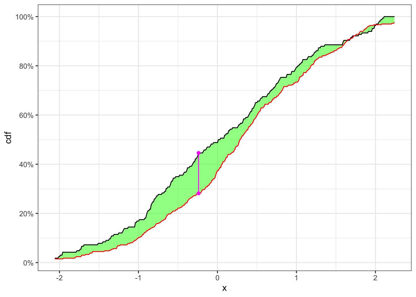
| \(\textbf{Index split}\) | \(\alpha\) | \(n_1\) | \(n_2\) | \(\text{KS}(\mathbf{x}_{n_1}, \mathbf{x}_{n_2})\) | p.value | \(\textbf{Critical level}\) | \(\mathcal{H}_0\) |
|---|---|---|---|---|---|---|---|
| 166 | 0.05 | 166 | 334 | 0.1643 | 0.002503 | 0.129 | Rejected |