The expectation of a random variable is it’s first moment, also called statistical average. In general, it is denoted as . Let’s consider a discrete random variable with distribution function . Then the expectation of is the weighted average between all the possible -states that the random variable can assume by it’s respective probability of occurrence, i.e. In the continuous case, i.e. when takes values in and admits a density function, the expectation is computed as an integral, i.e.
10.1.1 Sample statistic
Let’s consider a sample of IID observations, i.e. . Then the sample expectation is computed as:
Population vs sample
In general, the notation refers to a finite sample, e.g. is the sample mean. Instead the notation without , i.e. , stands for the random variable in population, e.g. is the mean in population. A population can be finite or non-finite. In the case of a finite population with element it is useful to distinguish between:
Extraction with reimmission of elements for the sample gives possible combinations.
Extraction without readmission of elements for the sample gives possible combinations.
Table 10.1: Expectation in a discrete and continuous population and in a sample .
Population (continuous)
Population (discrete)
Sample
10.1.2 Sample moments
Let’s consider an the moments of the sample mean of an IID sample. Since all the variables has the same expected value, i.e. , the expected value of the sample mean is computed as: The variance of the sample mean is computed as:
10.1.3 Sample distribution
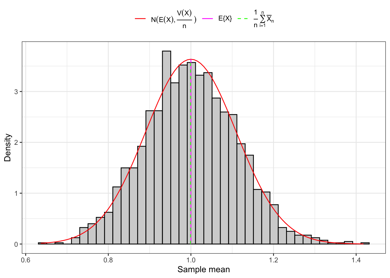
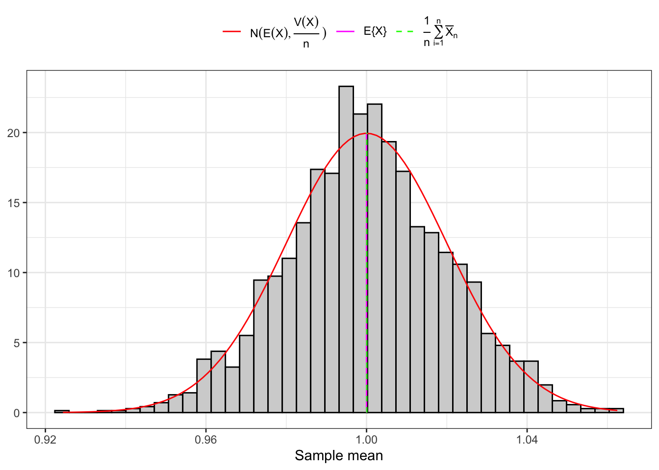
Proposition 10.1 Let’s consider a sample of IID random variables. If is sufficiently large, independently from the distribution of the , by the central limit theorem (CLT) the distribution of the sample expectation converges to the distribution of a normal random variable, i.e.
Proof. In order to prove Proposition 10.1 it is useful to compute the expectation and the variance of the following random variable, i.e. The expectation and the variance of can be easily obtained from Equation 10.1 and Equation 10.2 respectively and read: Applying the central limit theorem (Theorem 8.1) one obtain: Hence the random variable mean on large samples is distributed as a normal random variable, i.e. Note that on small sample this results holds true if and only if is normally distributed also in population. Under normality also in population we have that independently from the sample size:
Distribution of sample mean
# True population moments true <-c(e_x =1, v_x =2)# Number of elements for large samplesn <-5000# Number of elements for small samplesn_small <-trunc(n/30)# Number of sample to simulate n_sample <-2000# Simulation of sample meansstat_sample_small <-c()stat_sample_large <-c()for(i in1:n_sample){set.seed(i)# Large sample x_n <- true[1] +sqrt(true[2])*rnorm(n)# Statistic stat_sample_large[i] <-mean(x_n)# Small sample x_n <- x_n[1:n_small]# Statistic stat_sample_small[i] <-mean(x_n)}
(a) Small sample (166).
(b) Large sample (5000).
Figure 10.1: Distribution of the sample mean.
10.2 Variance and covariance
In general the variance of a random variable in population defined as: Let’s consider a discrete random variable with distribution function . Then the variance of is the weighted average between all the possible -centered and squared states that the random variable can assume by it’s respective probability of occurrence, i.e. In the continuous case, i.e. when admits a density function and takes values in , the expectation is computed as: Let’s consider two random variables and . Then, in general their covariance is defined as: In the discrete case where and have a joint distribution , their covariance is defined as: In the continuous case, if the joint distribution of and admits a density function the covariance is computed as:
10.2.1 Properties
There are several properties connected to the variance.
The variance can be computed as:
The variance is invariant with respect to the addition of a constant , i.e.
The variance scales upon multiplication with a constant , i.e.
The variance of the sum is computed as:
The covariance can be expressed as:
The covariance scales upon multiplication with a constant and , i.e.
Proof: Properties of the variance
Proof. The property 1. (Equation 10.3) follows easily developing the definition of variance, i.e. The property 2. (Equation 10.4) follows from the definition, i.e. The property 3. (Equation 10.5) follows using the expression of the variance in Equation 10.3, i.e. The property 4. (Equation 10.6), i.e. the variance of the sum of two random variables is: where in the case in which there is no linear connection between and the covariance is zero, i.e. . Developing the computation of the covariance it is possible to prove property 5. (Equation 10.7), i.e. Finally, using the result in property 5. (Equation 10.7) the result in property 6. (Equation 10.8) follows easily:
10.2.2 Conditional variance
Proposition 10.2 ()
Let’s consider two random variable and with finite second moment. Then, the total variance can be expressed as:
Proof. By definition, the variance of a random variable reads: Applying the tower property we can write Then, add and subtract , Grouping the first and fourth terms and the second and third one obtain
10.2.3 Sample statistic
The sample’s variance on is computed as: Equivalently, in terms of the first and second moment: In general, the variance computed as in Equation 10.9 is not correct for the population value. Hence, to correct the estimator let’s define the corrected sample’s variance:
10.2.4 Sample moments
Let’s consider an the moments of the sample variance on an IID sample. The expected value of the corrected sample variance: The variance of the corrected sample variance is: where is the kurtosis of . If the population is normal, and the variance simplifies in:
10.2.5 Sample distribution
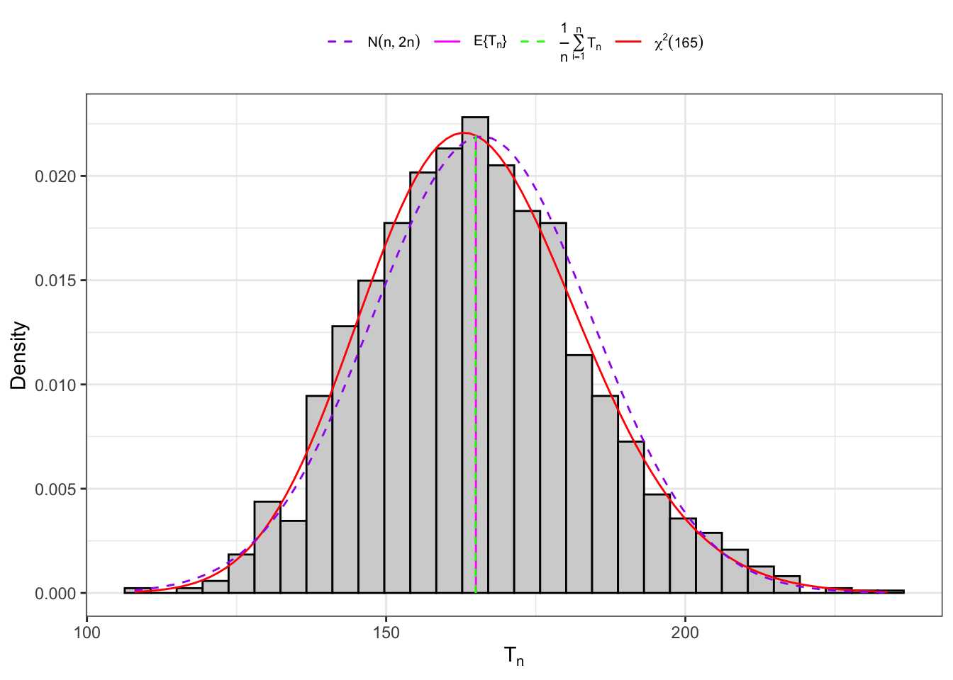
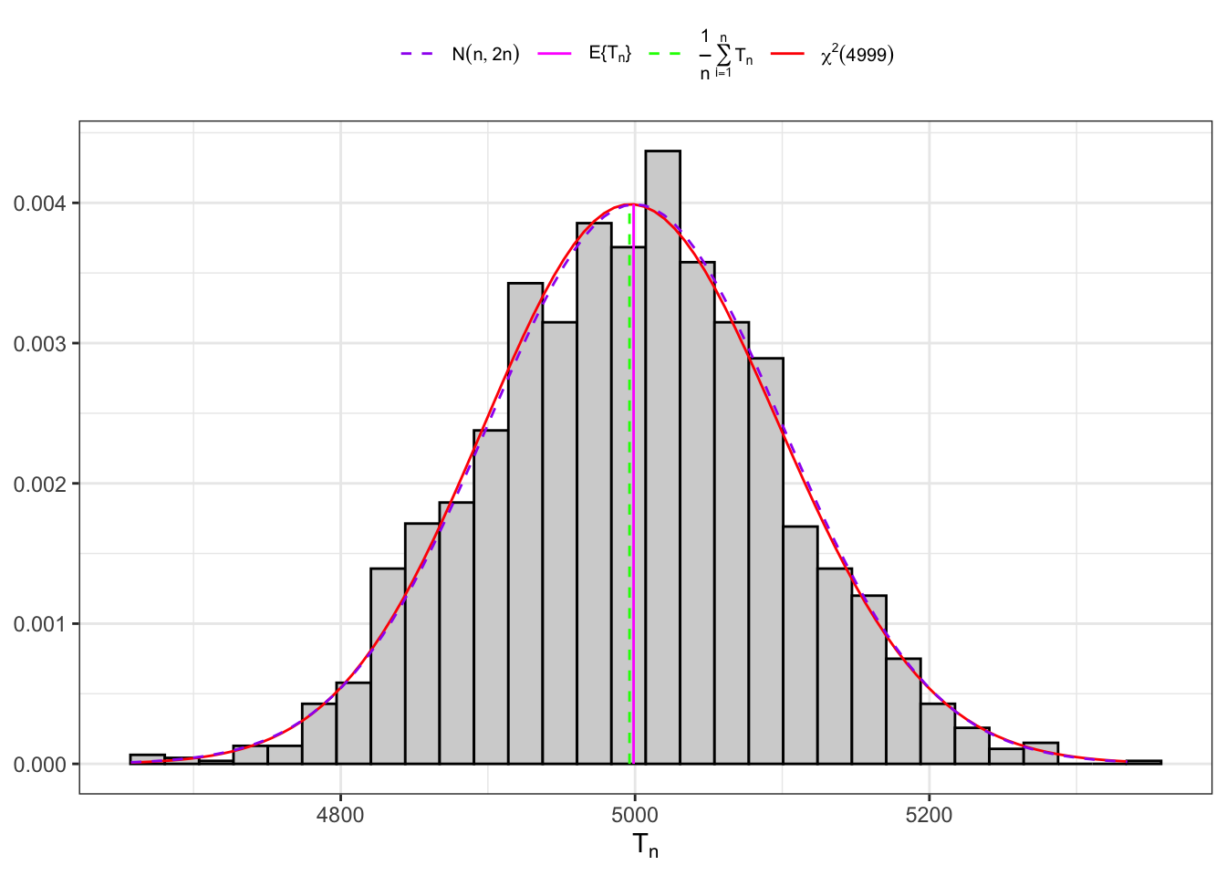
The distribution of the sample variance is available when we consider the sum of n-IID standard normal random variables. Notably, from Cochran’s theorem: Going to the limit as a random variable converges to a standard normal random variable, i.e. therefore, on large samples the statistic converges to a normal random variable, i.e.
Distribution of under normality.
If the population is normal, then the distribution of is proportional to the distribution of a . In fact, from Equation 10.15 the expectation of is: Similarly, computing the variance of Equation 10.15 and knowing that one obtain:
Distribution of under normality
# True population moments true <-c(e_x =1, v_x =2)# Number of elements for large samplesn <-5000# Number of elements for small samplesn_small <-trunc(n/30)# Number of sample to simulate n_sample <-2000# Simulation of sample variancestat_sample_small <-c()stat_sample_large <-c()for(i in1:n_sample){set.seed(i)# Large sample x_n <- true[1] +sqrt(true[2])*rnorm(n)# Statistic stat_sample_large[i] <- (1/(n-1))*sum((x_n -mean(x_n))^2)# Small sample x_n <- x_n[1:n_small]# Statistic stat_sample_small[i] <- (1/(n_small-1))*sum((x_n -mean(x_n))^2)}
(a) Small sample (166).
(b) Large sample (5000).
Figure 10.2: Distribution of the statistic under normality.
10.3 Skewness
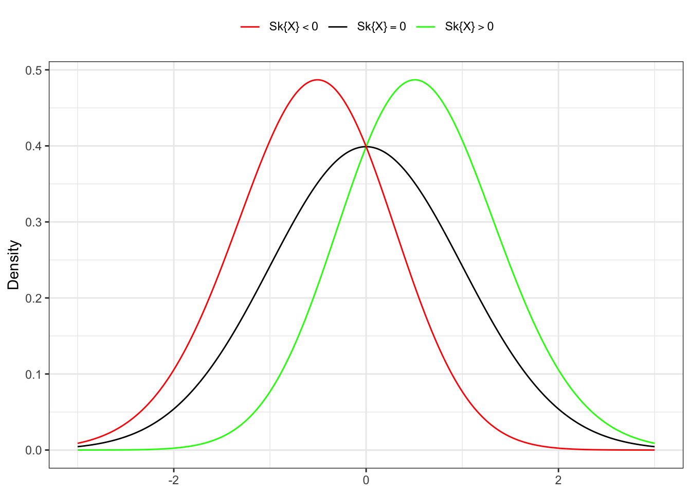
The skewness is a measure of the asymmetry of the probability distribution of a real-valued random variable about its mean. The skewness value can be positive, zero, negative, or undefined. For a uni modal distribution, negative skew commonly indicates that the tail is on the left side of the distribution, and positive skew indicates that the tail is on the right.
Figure 10.3: Skewness of a random variable.
Following the same notation as in Ralph B. D’agostino and Jr. (1990), let’s define and denote the population skewness of a random variable as:
10.3.1 Sample statistic
Let’s consider an IID sample , then the sample’s skewness is estimated as: The estimator in Equation 10.17 is not correct. Hence, let’s define the correct sample estimator of the skewness as:
10.3.2 Sample moments
Under normality, the asymptotic moments of the sample skewness are: In Urzúa (1996) are also reported the exact mean of the estimator in Equation 10.17 for small normal samples, i.e. and variance
10.3.3 Sample distribution
Under normality, the asymptotic distribution of the sample skewness is normal i.e.
10.4 Kurtosis
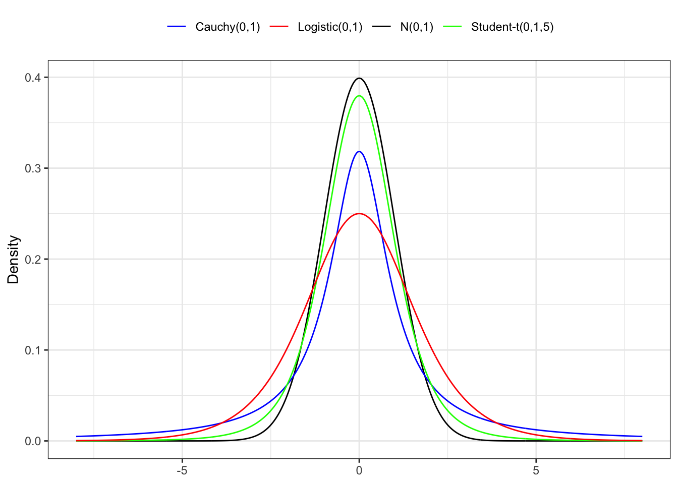
The kurtosis is a measure of the tailedness of the probability distribution of a real-valued random variable. The standard measure of a distribution’s kurtosis, originating with Karl Pearson is a scaled version of the fourth moment of the distribution. This number is related to the tails of the distribution. For this measure, higher kurtosis corresponds to greater extremity of deviations from the mean (or outliers). In general, it is common to compare the excess kurtosis of a distribution with respect to the normal distribution (with kurtosis equal to 3). It is possible to distinguish 3 cases:
A negative excess kurtosis or platykurtic are distributions that produces less outliers than the normal. distribution.
A zero excess kurtosis or mesokurtic are distributions that produces same outliers than the normal.
A positive excess kurtosis or leptokurtic are distributions that produces more outliers than the normal.
Figure 10.4: Kurtosis of a different leptokurtic distributions.
Let’s define and denote the population kurtosis of a random variable as: or equivalently the excess kurtosis as .
10.4.1 Sample statistic
Let’s consider an IID sample , then the sample’s kurtosis is denoted as: From Pearson (1931), we have a correct the version of defined as:
10.4.2 Sample moments
Under normality, the asymptotic moments of the sample kurtosis are: Notably in Urzúa (1996) are reported also the exact mean and variance for a small normal sample, i.e. and the variance as:
10.4.3 Sample distribution
Under normality, the asymptotic distribution of the sample kurtosis is normal, i.e.
Ralph B. D’agostino, Albert Belanger, and Ralph B. D’agostino Jr. 1990. “A Suggestion for Using Powerful and Informative Tests of Normality.”The American Statistician 44 (4): 316–21. https://doi.org/10.1080/00031305.1990.10475751.