9  Introduction

9.1 Population and Sample

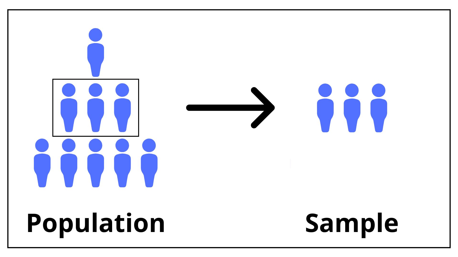
A population refers to the entire group of individuals or instances about whom we hope to learn. It encompasses all possible subjects or observations that meet a set of criteria. The population is the complete set of items that interest the researcher, and it can be finite (e.g. the students in a particular school) or infinite (e.g. the number of times a die can be rolled). A population size is given by the number of distinct elements and it includes every individual or observation of interest.

A sample is a subset of the population that is used to represent the population. Since studying an entire population is often impractical due to constraints like time, cost, and accessibility, samples provide a manageable and efficient way to gather data and make inferences about the population. It is important that the sample is representative of the population of interest to allow for valid inferences. It is always important to distinguish between a random sample, e.g. a random group of students in 5th year from a school to make inference about the students at the 5th year of such school, and a convenience sample, e.g. a class of 5th year students who are easily accessible to the researcher, but that can be not representative of all the 5th year students in the school.

Aspect	Population	Sample
Definition	Entire group of interest	Subset of the population
Size	Large, potentially infinite	Small, manageable
Data Collection	Often impractical to study directly	Practical and feasible
Purpose	To understand the whole group	To make inferences about the population

Figure 9.1: Population vs sample.

9.2 Estimators

Let’s consider a statistical model depending on some unknown parameter $\theta$ contained in the sample space of parameters $\mathrm{\Theta }$, i.e. $\{P_{\theta }:\theta \in \mathrm{\Theta }\}$. Then, given an observed sample from the statistical model, $X_n=(x_1,\dots ,x_n)$, an estimator is a function that maps the sample space to a set of sample estimates. Formally, since $X_n$ is a collection of random variables, then also any estimator of $\theta$, as function of the sample, is a random variable, i.e.  $$X_n⟶\theta (X_n)⟶\hat{\theta }(X_n)\text{,}$$ where we input a sample $X_n$ to an estimator function $\theta (X_n)$ and we output an estimate $\hat{\theta }(X_n)$. When we condition to a particular value of the sample $X_n$, we obtain a point estimate of the true $\theta$, i.e.  $$\hat{\theta }(X_n=(x_1,\dots ,x_n))=\hat{\theta }\text{,}$$ that is a number (or a vector).

Since the estimator is a random variable itself, one can define some metrics to compare different estimators of the same parameter. Firstly, let’s consider the bias, the distance between the average of the collection of estimates and the single parameter being estimated, i.e. $$\mathrm{Bias}\{\hat{\theta }(X_n)\}=\mathbb{E}\{\hat{\theta }(X_n)\}-\theta \text{.}$$ We distinguish between two kind of estimators:

• Biased, when $\mathrm{Bias}\{\hat{\theta }(X_n)\}\ne 0$.
• Unbiased, when $\mathrm{Bias}\{\hat{\theta }(X_n)\}=0$.

The variance is used to indicate how far the collection of estimates are from the expected value of the estimates, i.e. $$\mathbb{V}\{\hat{\theta }(X_n)\}=\mathbb{E}\left\{{(\hat{\theta }(X_n)-\mathbb{E}\{\hat{\theta }(X_n)\})}^2\right\}\text{.}$$ Finally, we have the Mean Squared Error (MSE) of an estimator, i.e.  $$\mathrm{MSE}\{\hat{\theta }(X_n)\}=\mathrm{Bias}\{\hat{\theta }(X_n){\}}^2+\mathbb{V}\{\hat{\theta }(X_n)\}\text{,}$$ where for an unbiased estimator, the mean squared error equals the variance.

9.2.1 Properties

As for some desirable property of an estimator one have

Consistency (weak): Definition 8.3 $$\hat{\theta }(X_n)\underset{n\to \mathrm{\infty }}{\stackrel{\mathbb{P}}{⟶}}\theta$$

Efficiency: Among unbiased estimators, one with minimal variance is called (finite-sample) efficient; asymptotically efficient means it attains the Cramér–Rao lower bound (CRLB) limit.

Asymptotic normality: for some normalizing sequence $a_n$ Definition 8.5 $$a_n(\hat{\theta }(X_n)-\theta )\underset{n\to \mathrm{\infty }}{\stackrel{d}{⟶}}\mathcal{N}(0,{\sigma }^2(\theta ))$$ for some normalizing sequence $a_n$.

9.2.2 Sufficiency and Completeness

Theorem 9.1 A statistic $T=T(X_n)$ is sufficient for $\theta$ iff the joint likelihood factors as $ $$f(X_n\mid \theta )=g(T(X_n)\mid \theta )h(X_n)$$

Theorem 9.2 Rao–Blackwell. If $T$ is sufficient and $\tilde{\tau }$ is any estimator, then $\hat{\tau }=\mathbb{E}[\tilde{\tau }\mid T]$ has $\mathrm{Var}(\hat{\tau })\le \mathrm{Var}(\tilde{\tau })$ and the same mean.

A statistic $T$ is complete if ${\mathbb{E}}_{\theta }[g(T)]=0$ for all $\theta$ implies $g(T)=0$ almost surely.

:::{#thm-lehmann–scheffe .thm} Lehmann–Scheffé. If $T$ is complete and sufficient and $\hat{\tau }=\mathbb{E}[\tilde{\tau }\mid T]$ is unbiased, then $\hat{\tau }$ is the unique UMVU (uniformly minimum-variance unbiased) estimator of $\tau (\theta )$. :::

9.2.3 Methods of construction

• Method of Moments (MoM): Solve sample moments $m_k=\frac{1}{n}\sum X_i^k$ for parameters matching population moments.

• Maximum Likelihood (MLE): Maximize $\ell (\theta )=\sum \log f(X_i;\theta )$. Properties: invariance ($g(\hat{\theta })$ estimates $g(\theta )$), consistency, asymptotic normality $\mathcal{N}(\theta ,I(\theta {)}^{-1}/n)$ under regularity.

• Rao–Blackwellization: Improve any unbiased estimator by conditioning on a sufficient statistic; with completeness, obtain UMVU (Lehmann–Scheffé).