A statistical hypothesis is a claim about the value of a parameter or population characteristic. In any hypothesis-testing problem, there are always two competing hypotheses under consideration
The null hypothesis\(\mathcal{H}_0\) representing the status quo.
The alternative hypothesis\(\mathcal{H}_1\) representing the research.
The objective of hypothesis testing is to decide, based on sample information, if the alternative hypothesis is actually supported by the data. One usually does new research to challenge the existing beliefs.
Is there strong evidence for the alternative?
Let’s consider that you want to establish if the null hypothesis\(\mathcal{H}_0\) is not supported by the data. One usually assumes to work under \(\mathcal{H}_0\); then, if the sample does not strongly contradict \(\mathcal{H}_0\), we will continue to believe in the plausibility of the null hypothesis. There are only two possible conclusions: Reject \(\mathcal{H}_0\) or Fail to reject \(\mathcal{H}_0\).
Definition 12.1 The test statistic\(T(\mathbf{x}_n)\) is a function of a sample and is used to make a decision about whether the null hypothesis should be rejected or not. In theory, there is an infinite number of possible tests that could be devised. The choice of a particular test procedure must be based on the probability that the test will produce incorrect results. In general, two kinds of errors are related to test statistics, i.e.
A type I error is when the null hypothesis is rejected, but it is true.
A type II error is not rejecting the null when it is false.
The p-value is the probability, computed under \(\mathcal{H}_0\), of observing a test statistic at least as extreme as the one obtained from the sample. The smaller the p-value, the stronger the evidence in the sample data against the null hypothesis and in favor of the alternative hypothesis.
In general, before performing a test one establishes a significance level \(\alpha\) (the desired type I error probability), which defines the rejection region. Then the decision rule is: \[
\begin{aligned}
{}
& \text{Reject } \mathcal{H}_0 && \iff \text{p-value } \le \alpha \\
& \text{Do not reject } \mathcal{H}_0 && \iff \text{p-value } > \alpha \\
\end{aligned}
\] The p-value can be thought of as the smallest significance level at which \(\mathcal{H}_0\) can be rejected, and its calculation depends on whether the test is upper, lower, or two-tailed.
For example, let’s consider a sample \(\mathbf{x}_n\) of data. Then, the general procedure for a statistical hypothesis test can be summarized as follows:
an assumption about the distribution of the data, often expressed in terms of a statistical model;
a null hypothesis \(\mathcal{H}_0\) and an alternative hypothesis \(\mathcal{H}_1\) which make specific statements about the data;
a test statistic \(T(\mathbf{x}_n)\) which is a function of the data and whose distribution under the null hypothesis is known;
a significance level \(\alpha\) which imposes an upper bound on the probability of rejecting \(\mathcal{H}_0\), given that \(\mathcal{H}_0\) is true.
Given that \(T(\mathbf{X}_n)\) under \(\mathcal{H}_0\) has a known distribution function \(F_{T}\), then the value \(q_{\alpha}\) is computed with the quantile function \(F^{-1}_{T}\) that is such that \[
F_{T}: \mathbb{R} \to [0, 1] \iff F^{-1}_{T}: [0, 1] \to \mathbb{R}
\text{.}
\] Mathematically, the p-value is related to the test performed. In general, two kinds of tests are available:
A two-tailed test is appropriate if the estimated value can depart from the reference value in both directions. For a continuous and symmetric statistic, if \(t_{\text{obs}}\) is the observed value, the p-value is \[
\text{p-value} = \mathbb{P}(|T(\mathbf{X}_n)| \ge |t_{\text{obs}}| \mid \mathcal{H}_0)
\text{.}
\] The two critical tails of a level-\(\alpha\) test are defined by \[
\mathbb{P}(T(\mathbf{X}_n) \le q_{\alpha/2}) = \frac{\alpha}{2}
\text{,} \quad \text{and} \quad
\mathbb{P}(T(\mathbf{X}_n) \ge q_{1 - \alpha/2}) = \frac{\alpha}{2}
\text{,}
\] where \(q_{\alpha/2} = F^{-1}_{T}(\alpha/2)\) and \(q_{1-\alpha/2} = F^{-1}_{T}(1-\alpha/2)\)
A one-tailed test is appropriate if the estimated value may depart from the reference value in only one direction, left or right, but not both. For a left-tailed test, the p-value is \(F_T(t_{\text{obs}})\) and the level-\(\alpha\) critical value satisfies \[
\mathbb{P}(T(\mathbf{X}_n) \le q_{\alpha}) = \alpha
\text{,}
\] while for a right-tailed test, the p-value is \(1-F_T(t_{\text{obs}})\) and the critical value satisfies \[
\mathbb{P}(T(\mathbf{X}_n) \ge q_{1 - \alpha}) = \alpha
\text{.}
\] If the distribution function is symmetric, then for a two-tailed test \(q_{\alpha/2} = -q_{1-\alpha/2}\) and the formulas simplify.
12.1 Tests for the means
Proposition 12.1 Let’s consider an IID, normally distributed sample, i.e. \(\mathbf{X}_n = (X_1, \dots, X_i, \dots, X_n)\) with \(X_i \sim \mathcal{N}(\mu, \sigma^2)\), and let’s consider the set of hypothesis \[
\mathcal{H}_0: \mu = \mu_0
\text{,}\quad
\mathcal{H}_1: \mu \neq \mu_0
\text{.}
\] Then, given the sample mean \(\hat{\mu}\) (Equation 10.1) and the corrected sample variance \(\hat{s}\) (Equation 10.6), under the null hypothesis \(\mathcal{H}_0\) the test statistic \[
T_n(\mathbf{X}_n) = \frac{\hat{\mu}(\mathbf{X}_n) - \mu_0}{\frac{\hat{s}(\mathbf{X}_n)}{\sqrt{n}}} \underset{\mathcal{H}_0}{\sim} t(n-1)
\text{,}
\] is Student-t distributed with \(n-1\) degrees of freedom. Moreover as \(n \to \infty\) the distribution of \(T(\mathbf{X}_n)\) converges (Definition 8.5) to the distribution of a Standard Normal, i.e. \[
T_n(\mathbf{X}_n) \overset{\text{d}}{\underset{\mathcal{H}_0}{\longrightarrow}} \mathcal{N}(0,1)
\iff
\lim_{n\to \infty} F_{T_n}(t) = \Phi(t)
\text{,}
\] where \(\Phi(t)\) denotes the distribution of a standard normal.
Proof. If the sample is normally distributed, the sample mean is also normally distributed, i.e. \[
M(\mathbf{X}_n) = \sqrt{n}\frac{\hat{\mu}(\mathbf{X}_n) - \mu_0}{\sigma} \sim \mathcal{N}(0,1)
\text{.}
\] Under normality the sample variance, which is a sum of the squares of independent and normally distributed random variables, follows a \(\chi^2\) distribution with \(n-1\) degrees of freedom, i.e. \[
V(\mathbf{X}_n) = \frac{(n-1)\hat{s}^2(\mathbf{X}_n)}{\sigma^2} \sim \chi^2(n-1)
\text{.}
\] Notably, the ratio of a standard normal and a \(\chi^2\) random variable (the latter divided by its degrees of freedom) is exactly the definition of a Student-t random variable as in Equation 32.2. Hence, the ratio between the statistics \(M\) and \(V\) divided by their degrees of freedom reads \[
\frac{M(\mathbf{X}_n)}{\sqrt{\frac{V(\mathbf{X}_n)}{n-1}}} =
\sqrt{n} \frac{\hat{\mu}(\mathbf{X}_n) - \mu}{\sigma} \sqrt{\frac{\sigma^2}{\hat{s}^2(\mathbf{X}_n)}} = \sqrt{n} \frac{\hat{\mu}(\mathbf{X}_n) - \mu}{\hat{s}^2(\mathbf{X}_n)}
\sim t_{n-1}
\text{.}
\] The test statistic under \(\mathcal{H}_0\) follows a Student-t distribution with \(n-1\) degrees of freedom.
Exercise 12.1 Let’s consider a sample of \(n = 500\) IID random variables, where each observation is drawn from a normal distribution with mean \(\mu = 2\) and variance \(\sigma^2 = 4\). Then, evaluate, with an appropriate test, if the following three sets of hypotheses are statistically significant with significance level \(\alpha = 10\%\), i.e. \[
\begin{aligned}
{} & \text{(1)} &&
\mathcal{H}_0: \mu = 2.3
\text{,} &&
\mathcal{H}_1: \mu \neq 2.3 \text{,} \\
& \text{(2)} &&
\mathcal{H}_0: \mu = 2.2
\text{,} &&
\mathcal{H}_1: \mu \neq 2.2 \text{,} \\
& \text{(3)} &&
\mathcal{H}_0: \mu = 2.1
\text{,} &&
\mathcal{H}_1: \mu \neq 2.1 \text{.} \\
\end{aligned}
\]
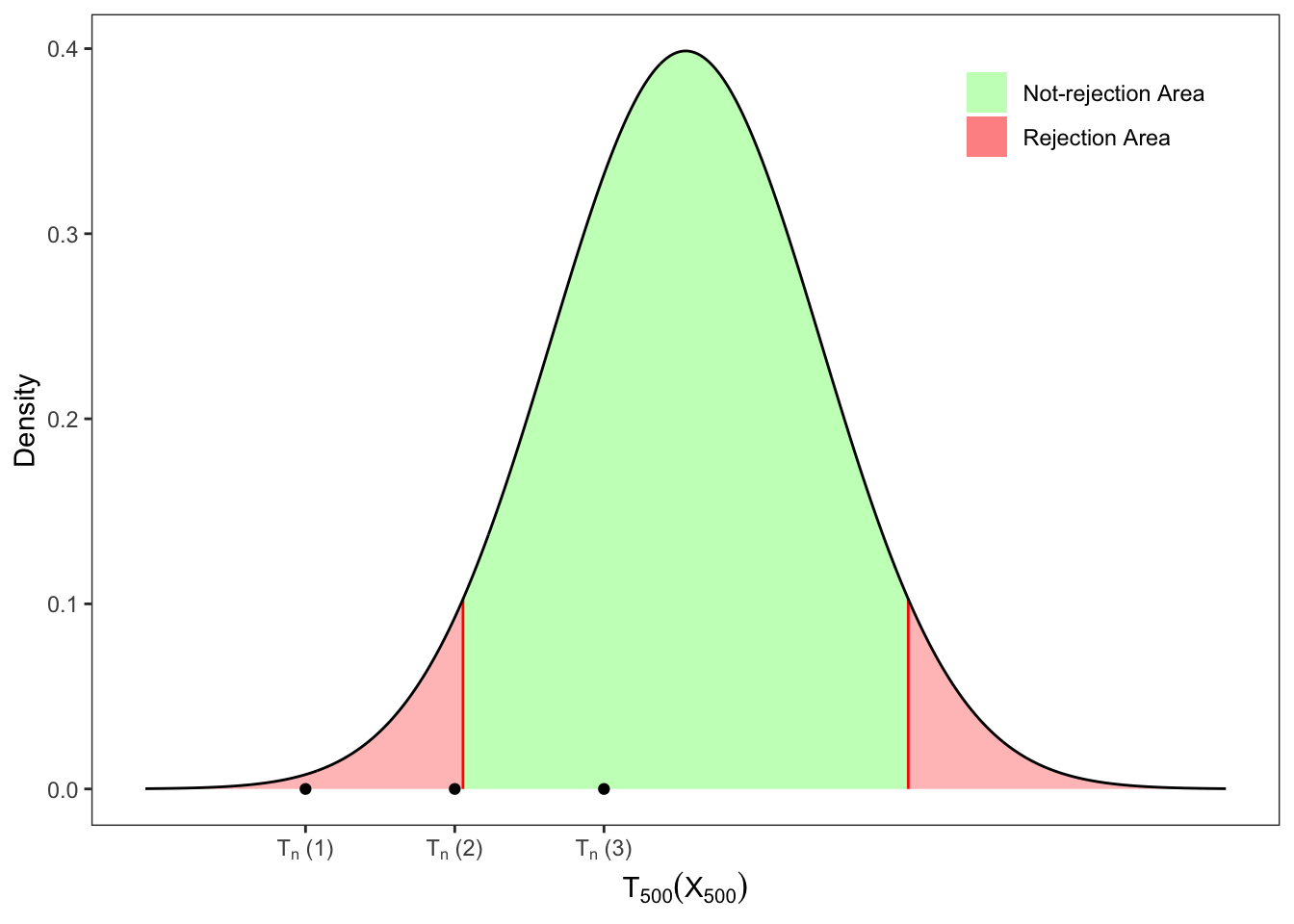
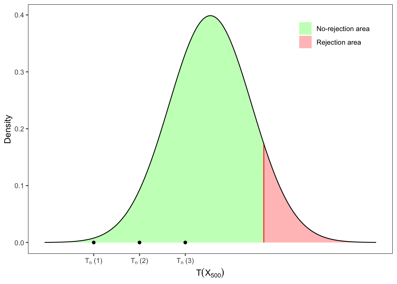
Solution 12.1. Since we are dealing with a single Normal population, we can apply a t-test (Proposition 12.1). More precisely, the statistic will be Student-t distributed and the critical value with probability \(\alpha\) is such that: \[
q_{\alpha/2} = F_{T_n}^{-1}(\alpha/2) \text{,}
\] where \(F_{T_n}^{-1}\) is the quantile function of a Student-t. Therefore, if the statistic computed on a sample \(\mathbf{x}_n\) lies inside the non-rejection area, i.e. \[
\mathcal{H}_0 \text{ is not rejected} \iff
-|q_{\alpha /2}| < T_n(\mathbf{x}_n) < |q_{\alpha /2}|
\text{,}
\] then we do not reject \(\mathcal{H}_0\) with probability \(\alpha\) and we cannot conclude that the mean is significantly different from \(\mu_0\).
Solution
library(dplyr)set.seed(1) # random seed# ============================================# Inputs# ============================================# Dimension of the samplen <-500# number of simulations# Means for the testsmu_0 <-c(2.3, 2.2, 2.1)# true meanmu <-2# true variancesigma2 <-4alpha <-0.1# significance level# ============================================# Simulated random variablex <-rnorm(n, mean = mu, sd =sqrt(sigma2))# Sample meanmu_hat <-mean(x)# Corrected sample variances2_hat <- (mean(x^2) - mu_hat^2) * n / (n -1)# Statistic T (1)T_1 <-sqrt(n) * (mu_hat - mu_0[1]) /sqrt(s2_hat)# Statistic T (2)T_2 <-sqrt(n) * (mu_hat - mu_0[2]) /sqrt(s2_hat)# Statistic T (3)T_3 <-sqrt(n) * (mu_hat - mu_0[3]) /sqrt(s2_hat)# Degrees of freedomnu <- n -1# Critical valueq_alpha_2 <-abs(qt(alpha /2, df = nu))
\(\mu_0\)
\(\alpha\)
\(q_{\alpha/2}\)
\(T_n(\mathbf{x}_{n})\)
\(q_{1-\alpha/2}\)
\(\mathcal{H}_0\)
2.3
0.1
-1.648
-2.814
1.648
Rejected
2.2
0.1
-1.648
-1.709
1.648
Rejected
2.1
0.1
-1.648
-0.604
1.648
Not-rejected
Table 12.1: t-tests on the mean of a Normal sample.
Figure 12.1: t-tests on the mean of a Normal sample.
12.1.1 Test for two means and equal variances
Proposition 12.2 Let’s consider two IID Gaussian samples with unknown means \(\mu_1\) and \(\mu_2\) and unknown equal variances \(\sigma_1^2 = \sigma_2^2 = \sigma^2\), i.e. \[
\mathbf{X}_{n_1} \sim \mathcal{N}(\mu_1, \sigma^2), \quad \mathbf{X}_{n_2} \sim \mathcal{N}(\mu_2, \sigma^2)
\text{,}
\] where \(n_1\) and \(n_2\) are the number of observations in each sample and let’s consider the set of hypotheses \[
\mathcal{H}_0: \mu_1 - \mu_2 = \mu_{\Delta}
\text{,}\quad
\mathcal{H}_1: \mu_1 - \mu_2 \neq \mu_{\Delta}
\text{.}
\] Then, given the sample mean \(\hat{\mu}(\mathbf{x}_n)\) (Equation 10.1) under the null hypothesis \(\mathcal{H}_0\) the test statistic is Student-t distributed with \(n_1 + n_2 - 2\) degrees of freedom, i.e. \[
T(\mathbf{X}_{n_1}, \mathbf{X}_{n_2}) = \frac{\hat{\mu}(\mathbf{X}_{n_1}) - \hat{\mu}(\mathbf{X}_{n_2}) - \mu_{\Delta}}{\sqrt{\hat{s}^2(\mathbf{X}_{n_1}, \mathbf{X}_{n_2})}}
\underset{\mathcal{H}_0}{\sim}
\text{t}(n_1 + n_2 - 2)
\text{,}
\tag{12.1}\] where \[
\hat{s}^2(\mathbf{X}_{n_1}, \mathbf{X}_{n_2}) = \frac{(n_1 - 1)\hat{s}^2(\mathbf{X}_{n_1}) + (n_2 - 1)\hat{s}^2(\mathbf{X}_{n_2})}{n_1 + n_2 - 2} \left(\frac{1}{n_1} + \frac{1}{n_2}\right)
\text{,}
\tag{12.2}\] and \(\hat{s}^2\) is the sample corrected variance (Equation 10.6) computed on the two samples.
Exercise 12.2 Let’s consider two samples extracted from a Normal distribution with \(n_1 = 100\) and \(n_2 = 200\) and \[
\mathbf{X}_{100} \sim \mathcal{N}(2, 4), \quad \mathbf{X}_{200} \sim \mathcal{N}(1, 4)
\text{,}
\] Then, let’s evaluate with an appropriate test and significance level \(\alpha = 10\%\) the following sets of hypotheses, i.e. \[
\begin{aligned}
{} & \text{(1)} &&
\mathcal{H}_0: \mu_{\Delta} = \mu_1 - \mu_2 = 0.5
\text{,} &&
\mathcal{H}_1: \mu_{\Delta} = \mu_1 - \mu_2\neq 0.5 \text{,} \\
& \text{(2)} && \mathcal{H}_0: \mu_{\Delta} = \mu_1 - \mu_2 = 0.75
\text{,}
&& \mathcal{H}_1: \mu_{\Delta} = \mu_1 - \mu_2 \neq 0.75 \text{,} \\
& \text{(3)} && \mathcal{H}_0: \mu_{\Delta} = \mu_1 - \mu_2 = 1
\text{,}
&& \mathcal{H}_1: \mu_{\Delta} = \mu_1 - \mu_2 \neq 1 \text{,}
\end{aligned}
\]
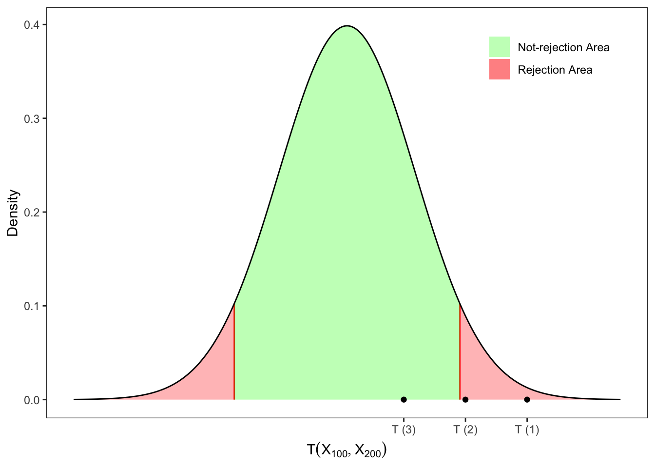
Solution 12.2. Since the samples are normally distributed in populations with equal variances, we can consider the test statistic in Equation 12.1. More precisely, the test statistic is Student-t distributed \[
T(\mathbf{x}_{100}, \mathbf{x}_{200}) = \frac{\hat{\mu}(\mathbf{x}_{100}) - \hat{\mu}(\mathbf{x}_{200}) - \mu_{\Delta}}{\sqrt{\hat{s}^2(\mathbf{x}_{100}, \mathbf{x}_{200})}}
\underset{\mathcal{H}_0}{\sim}
t_{298}
\text{,}
\] where \(\hat{s}^2(\mathbf{x}_{100}, \mathbf{x}_{200})\) is computed as in Equation 12.2. Since it is a two-tailed test the critical value for a significance level \(\alpha\) is defined as the value of the statistic \[
q_{\alpha/2} = F_{T}^{-1}(\alpha/2)
\text{,}
\] where \(F_{T}^{-1}\) is the quantile function of a Student-t, which is symmetric. Therefore, if \(T\) lies inside the non-rejection area, i.e. \[
\mathcal{H}_0 \text{ is not rejected} \iff
-|q_{\alpha /2}|
< T(\mathbf{x}_n) <
|q_{\alpha /2}|
\text{,}
\] then \(\mathcal{H}_0\) is not rejected with probability \(\alpha\) and one cannot conclude that the difference between the sample means is significantly different from \(\mu_{\Delta}\). Otherwise, when \(\mathcal{H}_0\) is rejected, one can conclude that the difference between the sample means is statistically different from \(\mu_{\Delta}\).
Table 12.2: Tests on the difference between the means of two Normal populations with equal variances.
Figure 12.2: Tests on the difference between the means of two Normal populations with equal variances.
12.1.2 Test for two means and unequal variances
Proposition 12.3 Let’s consider two IID Gaussian samples with unknown means \(\mu_1\) and \(\mu_2\) and unknown variances \(\sigma_1^2\) and \(\sigma_2^2\), i.e. \[
\mathbf{X}_{n_1} \sim \mathcal{N}(\mu_1, \sigma_1^2), \quad \mathbf{X}_{n_2} \sim \mathcal{N}(\mu_2, \sigma_2^2)
\text{,}
\] where \(n_1\) and \(n_2\) are the number of observations in each sample and let’s consider the set of hypotheses \[
\mathcal{H}_0: \mu_1 - \mu_2= \mu_{\Delta}
\text{,}\quad
\mathcal{H}_1: \mu_1 - \mu_2 \neq \mu_{\Delta}
\text{.}
\] Then, given the sample means \(\hat{\mu}\) (Equation 10.1) and corrected sample variances (Equation 10.6), Welch (1938) - Welch (1947) proposes a test statistic that under the null hypothesis \(\mathcal{H}_0\) is approximately Student-t distributed with \(\nu\) degrees of freedom, i.e. \[
T(\mathbf{X}_{n_1}, \mathbf{X}_{n_2}) =
\frac{\hat{\mu}(\mathbf{X}_{n_1}) - \hat{\mu}(\mathbf{X}_{n_2})- \mu_{\Delta}}{\sqrt{\frac{\hat{s}^2(\mathbf{X}_{n_1})}{n_1} + \frac{\hat{s}^2(\mathbf{X}_{n_2})}{n_2}}}
\underset{\mathcal{H}_0}{\sim}
t_{\nu}
\text{,}
\] where the degrees of freedom \(\nu\) is not necessarily an integer and it is computed using the Welch-Satterthwaite approximation. More precisely, it is defined as a weighted average of the degrees of freedom of each group, reflecting the uncertainty due to unequal variances, i.e. \[
\nu = \frac{\left( \frac{\hat{s}^2(\mathbf{X}_{n_1})}{n_1} + \frac{\hat{s}^2(\mathbf{X}_{n_1})}{n_2} \right)^2}{\frac{(\hat{s}^2(\mathbf{X}_{n_1}))^2}{n_1^2 (n_1 - 1)} + \frac{(\hat{s}^2(\mathbf{X}_{n_1}))^2}{n_2^2(n_2 - 1)}}
\text{.}
\]
Exercise 12.3 Let’s consider two samples extracted from a Normal distribution with \(n_1 = 100\) and \(n_2 = 200\) and \[
\mathbf{X}_{100} \sim \mathcal{N}(2, 4), \quad \mathbf{X}_{200} \sim \mathcal{N}(1, 9)
\text{,}
\] Then, let’s evaluate with an appropriate test and significance level \(\alpha = 10\%\) the following sets of hypotheses in Exercise 12.2.
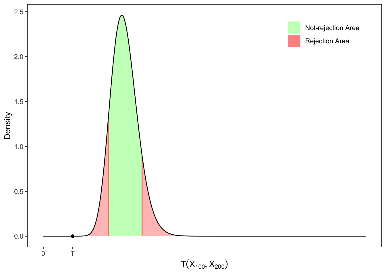
Table 12.3: Tests on the difference between the means of two Normal populations with unequal variances.
Figure 12.3: Tests on the difference between the means of two Normal populations with unequal variances.
12.2 Tests for the variances
12.2.1 F-test for two variances
Proposition 12.4 Let’s consider two IID Gaussian samples with unknown means \(\mu_1\) and \(\mu_2\) and unknown variances \(\sigma_1^2\) and \(\sigma_2^2\), i.e. \[
\mathbf{X}_{n_1} \sim \mathcal{N}(\mu_1, \sigma_1^2), \quad \mathbf{X}_{n_2} \sim \mathcal{N}(\mu_2, \sigma_2^2)
\text{,}
\] where \(n_1\) and \(n_2\) are the number of observations in each sample and let’s consider the set of hypotheses \[
\mathcal{H}_0: \sigma^2_1 = \sigma_2^2 = \sigma^2
\text{,}\quad
\mathcal{H}_1: \sigma^2_1 \neq \sigma_2^2
\text{.}
\] Then, given the corrected sample variances (Equation 10.6), the following test statistic under the null hypothesis \(\mathcal{H}_0\) has a Fisher-Snedecor distribution (Equation 32.3) with \(n_1 -1\) and \(n_2 -1\) degrees of freedom, i.e. \[
T(\mathbf{X}_{n_1}, \mathbf{X}_{n_2}) \underset{\mathcal{H}_0}{\sim}
\frac{\hat{s}^2(\mathbf{X}_{n_1})}{\hat{s}^2(\mathbf{X}_{n_2})} \sim \text{F}(n_1 - 1, n_2 - 1)
\text{.}
\] This means that the null hypothesis of equal variances can be rejected when the statistic is as extreme or more extreme than the critical values obtained from the \(\text{F}\)-distribution with degrees of freedom \(n_1 - 1\) and \(n_2 - 1\) and significance level \(\alpha\), i.e. \[
\mathcal{H}_0 \text{ is not rejected} \iff q_{\alpha/2} \le T(\mathbf{x}_{n_1}, \mathbf{x}_{n_2}) \le q_{1-\alpha/2}
\text{.}
\]
Proof. Using the fact that the sample variance of a Normal IID population is \(\chi^2\)-distributed (Equation 10.10) let’s define the statistics \[
\begin{aligned}
{} & T_1(\mathbf{X}_{n_1}) = (n_1-1)\frac{\hat{s}^2(\mathbf{X}_{n_1})}{\sigma_1^2}
\sim \chi^2(n_1 - 1) \text{,} \\
& T_2(\mathbf{X}_{n_2}) = (n_2-1)\frac{\hat{s}^2(\mathbf{X}_{n_2})}{\sigma_2^2}
\sim \chi^2(n_2 - 1) \text{.} \\
\end{aligned}
\] where \(\hat{s}\) reads as in Equation 10.6. Hence, the statistic given by their ratios reads: \[
\begin{aligned}
T(\mathbf{X}_{n_1}, \mathbf{X}_{n_2}) {} & =
\frac{\frac{T_1(\mathbf{X}_{n_1})}{n_1 - 1}}{\frac{T_2(\mathbf{X}_{n_2})}{n_2 - 1}} = \frac{\frac{\hat{s}^2(\mathbf{X}_{n_1})}{\sigma^2_1}}{\frac{\hat{s}^2(\mathbf{X}_{n_2})}{\sigma^2_2} } = \frac{\hat{s}^2(\mathbf{X}_{n_1}) \sigma^2_2 }{\hat{s}^2(\mathbf{X}_{n_2}) \sigma^2_1}
\text{.}
\end{aligned}
\] Thus, using the fact that the ratio of two independent \(\chi^2\) random variables divided by their respective degrees of freedom follows an \(F\)-distribution (Equation 32.3) with \(n_1-1\) and \(n_2-1\) degrees of freedom, and that under \(\mathcal{H}_0: \sigma^2_1 = \sigma_2^2 = \sigma^2\) one obtains \[
T(\mathbf{X}_{n_1}, \mathbf{X}_{n_2}) =
\frac{\hat{s}^2(\mathbf{X}_{n_1})}{\hat{s}^2(\mathbf{X}_{n_2})}
\underset{\mathcal{H}_0}{\sim}
\text{F}(n_1 - 1, n_2 - 1)
\text{.}
\]
Exercise 12.4 Let’s consider two samples extracted from a Normal distribution with \(n_1 = 100\) and \(n_2 = 200\) and \[
\mathbf{X}_{100} \sim \mathcal{N}(2, 4.4), \quad \mathbf{X}_{200} \sim \mathcal{N}(1, 4)
\text{,}
\] Then, let’s evaluate with an appropriate test and significance level \(\alpha = 10\%\) the following sets of hypotheses, i.e. \[
\begin{aligned}
{} & \text{(1)} &&
\mathcal{H}_0: \sigma_1 = \sigma_2
\text{,} &&
\mathcal{H}_1: \sigma_1 \neq \sigma_2 \text{.}
\end{aligned}
\]
Table 12.4: Tests on the difference between the variances of two Normal populations.
Figure 12.4: Tests on the difference between the variances of two Normal populations.
12.3 Left and right tailed tests
Let’s consider the three kinds of tests that can be performed: two-tailed, left-tailed and right-tailed. Starting with the first one, in general it is used to evaluate if an estimate is equal or not to a certain value.
For example, consider an observed sample \(\mathbf{x}_n\), drawn from an IID population, and suppose we would like to investigate if it has a certain population mean \(\mu_0 = \mathbb{E}\{X_1\}\). In practice, in this setting we are considering the following set of hypotheses, i.e. \[
\mathcal{H}_0: \mu = \mu_0
\text{,}\quad
\mathcal{H}_1: \mu \neq \mu_0
\text{.}
\] where in general \(\mathcal{H}_0\) is what the researcher expects to be true, while \(\mathcal{H}_1\) is the complementary alternative. Given a statistic \(T\) that has a known distribution \(F_T\) under \(\mathcal{H}_0\), the critical value \(q_{\alpha/2}\) for a significance level \(\alpha\) is defined \[
\begin{aligned}
\alpha & {} = \mathbb{P}([T(\mathbf{X}_n) < q_{\alpha/2}] \cup [T(\mathbf{X}_n) > q_{1-\alpha/2}]) \\
\Updownarrow & \\
q_{\alpha/2} & = F_{T}^{-1}(\alpha/2) \text{,}\quad q_{1-\alpha/2} = F_{T}^{-1}(1-\alpha/2)
\end{aligned}
\] where \(F_{T}^{-1}\) is the quantile function. Therefore, if the test statistic lies in the rejection area, i.e. \[
T_n(\mathbf{X}_n) < q_{\alpha /2}
\quad \text{or}\quad
T_n(\mathbf{X}_n) > q_{1-\alpha /2}
\text{.}
\] then we reject \(\mathcal{H}_0\) at significance level \(\alpha\) and we can conclude that the mean is significantly different from \(\mu_0\).
Let’s now instead consider a one-tailed test, appropriate if the estimated value may depart from the reference value only in one direction, left or right, but not both. Let’s consider the set of hypotheses, \[
\mathcal{H}_0: \mu = \mu_0
\text{,}\quad
\mathcal{H}_1: \mu < \mu_0
\text{.}
\] In this case, we need a left-tailed test. The test statistic \(T\) can be left the same as in the two-tailed test, but the critical values now must be re-computed. In fact, in this case we will search for a \(q_{\alpha}\) such that \(\mathbb{P}(T \le q_{\alpha}) = \alpha\). Applying the quantile function we obtain: \[
\begin{aligned}
\alpha & {} = \mathbb{P}(T_n(\mathbf{X}_n) < q_{\alpha}) \\
\Updownarrow & \\
q_{\alpha} & = F^{-1}_{T}(\alpha) \text{,}
\end{aligned}
\] Therefore, if the test statistic lies in the rejection area, i.e. \[
T(\mathbf{X}_n) < q_{\alpha}
\text{.}
\] then we reject \(\mathcal{H}_0\) at significance level \(\alpha\) and we can conclude that the mean is significantly lower than \(\mu_0\).
Exercise 12.5 Continuing from Exercise 12.1, evaluate with a left-tailed test with significance level \(\alpha = 10\%\) the following sets of hypotheses, i.e. \[
\begin{aligned}
{} & \text{(1)} &&
\mathcal{H}_0: \mu = 2.3
\text{,} &&
\mathcal{H}_1: \mu< 2.3 \text{,} \\
& \text{(2)} &&
\mathcal{H}_0: \mu = 2.2
\text{,} &&
\mathcal{H}_1: \mu < 2.2 \text{,} \\
& \text{(3)} &&
\mathcal{H}_0: \mu = 2.1
\text{,} &&
\mathcal{H}_1: \mu < 2.1 \text{.} \\
\end{aligned}
\]
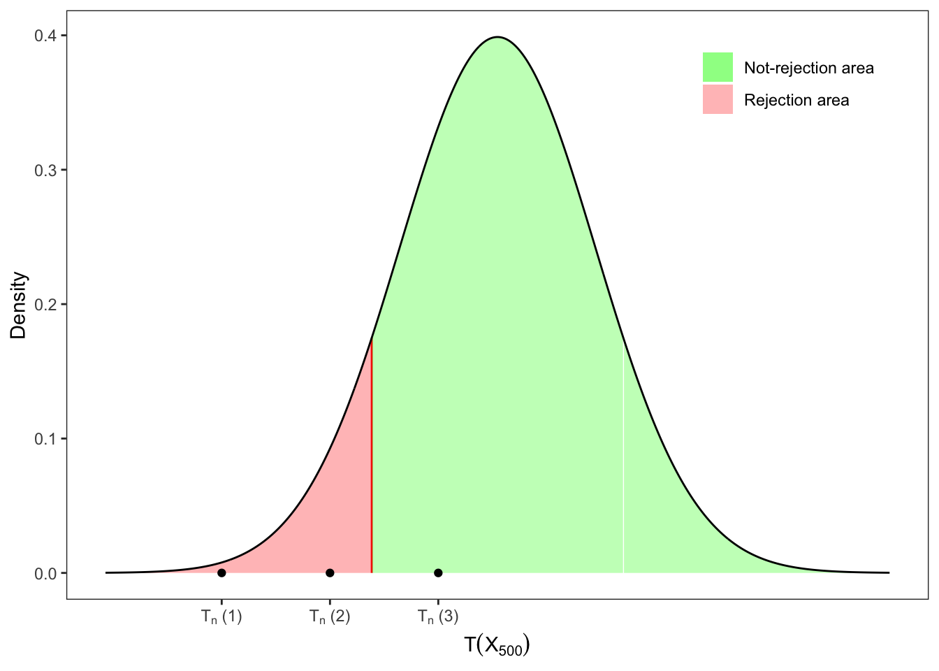
Solution 12.5. In this case, we need a left-tailed test. The test statistic \(T\) can be left the same as in Exercise 12.1, but the critical values now must be re-computed. In fact, in this case we will search for a \(q_{\alpha}\) such that \(\mathbb{P}(T \le q_{\alpha}) = \alpha\). Applying the quantile function we obtain: \[
q_{\alpha} = F^{-1}_{T}(\alpha)
\text{.}
\] In this case, with \(\alpha = 0.10\), the critical value of a Student-t with 499 degrees of freedom is \(q_{\alpha} = -1.28325\). Therefore, if \(T \ge -1.28325\) we do not reject the null hypothesis, i.e. \[
\mathcal{H}_0 \text{ is not rejected}
\iff
T_n(\mathbf{x}_n) \ge q_{\alpha}
\text{.}
\]
Solution
library(dplyr)set.seed(1) # random seed# ================== Setups ==================# Dimension of the samplen <-500# number of simulations# Means for the testsmu_0 <-c(2.3, 2.2, 2.1)# true meanmu <-2# true variancesigma2 <-4alpha <-0.1# significance level# ============================================# Simulated random variablex <-rnorm(n, mean = mu, sd =sqrt(sigma2))# Sample meanmu_hat <-mean(x)# Corrected sample variances2_hat <- (mean(x^2) - mu_hat^2) * n / (n -1)# Statistic T (1)T_1 <-sqrt(n) * (mu_hat - mu_0[1]) /sqrt(s2_hat)# Statistic T (2)T_2 <-sqrt(n) * (mu_hat - mu_0[2]) /sqrt(s2_hat)# Statistic T (3)T_3 <-sqrt(n) * (mu_hat - mu_0[3]) /sqrt(s2_hat)# Critical valueq_alpha <-qt(alpha, df = n -1)
\(\alpha\)
\(\mu_0\)
\(q_{\alpha}\)
\(T_n(\mathbf{x}_{n})\)
\(\mathcal{H}_0\)
0.1
2.3
-1.283
-2.814
Rejected
0.1
2.2
-1.283
-1.709
Rejected
0.1
2.1
-1.283
-0.604
Not-rejected
Table 12.5: Left-tailed t-tests on the mean of a Normal sample.
Figure 12.5: Left-tailed test on the mean.
Lastly, let’s consider the right-tailed test for the set of hypothesis \[
\mathcal{H}_0: \mu = \mu_0
\text{,}\quad
\mathcal{H}_1: \mu > \mu_0
\text{.}
\] It is still a one-sided test, but in this case the critical value \(q_{1-\alpha}\) is defined as \[
\begin{aligned}
\alpha & {} = 1 - \mathbb{P}(T(\mathbf{X}_n) \le q_{1-\alpha}) \\
\Updownarrow & \\
q_{1-\alpha} & = F^{-1}_{T}(1 - \alpha) \text{.}
\end{aligned}
\] Therefore, if the test statistic lies inside the non-rejection area, i.e. \[
\mathcal{H}_0 \text{ is not rejected}
\iff
T(\mathbf{x}_n) \le q_{1-\alpha}
\text{.}
\]
Exercise 12.6 Continuing from Exercise 12.1, evaluate with a right-tailed test with significance level \(\alpha = 10\%\) the following sets of hypotheses, i.e. \[
\begin{aligned}
{} & \text{(1)} &&
\mathcal{H}_0: \mu = 2.3
\text{,} &&
\mathcal{H}_1: \mu > 2.3 \text{,} \\
& \text{(2)} &&
\mathcal{H}_0: \mu = 2.2
\text{,} &&
\mathcal{H}_1: \mu > 2.2 \text{,} \\
& \text{(3)} &&
\mathcal{H}_0: \mu = 2.1
\text{,} &&
\mathcal{H}_1: \mu > 2.1 \text{.} \\
\end{aligned}
\]
Solution 12.6. It is still a one-sided test, but in this case the critical value \(q_{1-\alpha}\) is defined as \[
q_{1-\alpha} = F^{-1}_{T_n}(1 - \alpha)
\text{,}
\] In this case, with \(\alpha = 10\%\), the critical value of a Student-t with 499 degrees of freedom is \(q_{1-\alpha} = 1.28325\).
Therefore, if \(T \le 1.28325\) we do not reject the null hypothesis; otherwise, we reject it and conclude that the sample mean is greater than \(\mu_{0}\). Coherently with the previous test performed in Figure 12.5, a right-tailed test is never rejected.
Solution
library(dplyr)set.seed(1) # random seed# ================== Setups ==================# Dimension of the samplen <-500# number of simulations# Means for the testsmu_0 <-c(2.3, 2.2, 2.1)# true meanmu <-2# true variancesigma2 <-4alpha <-0.1# significance level# ============================================# Simulated random variablex <-rnorm(n, mean = mu, sd =sqrt(sigma2))# Sample meanmu_hat <-mean(x)# Corrected sample variances2_hat <- (mean(x^2) - mu_hat^2) * n / (n -1)# Statistic T (1)T_1 <-sqrt(n) * (mu_hat - mu_0[1]) /sqrt(s2_hat)# Statistic T (2)T_2 <-sqrt(n) * (mu_hat - mu_0[2]) /sqrt(s2_hat)# Statistic T (3)T_3 <-sqrt(n) * (mu_hat - mu_0[3]) /sqrt(s2_hat)# Critical valueq_alpha <-qt(1-alpha, df = n -1)
\(\alpha\)
\(\mu_0\)
\(T_n(\mathbf{x}_{n})\)
\(q_{1-\alpha}\)
\(\mathcal{H}_0\)
0.1
2.3
-2.814
1.283
Not-rejected
0.1
2.2
-1.709
1.283
Not-rejected
0.1
2.1
-0.604
1.283
Not-rejected
Table 12.6: Right-tailed t-tests on the mean of a Normal sample.
Figure 12.6: Right-tailed test on the mean.
Welch, B. L. 1938. “The Significance of the Difference Between Two Means When the Population Variances Are Unequal.”Biometrika 29 (3/4): 350–62. https://doi.org/10.1093/biomet/29.3-4.350.
———. 1947. “The Generalization of "Student’s" Problem When Several Different Population Variances Are Involved.”Biometrika 34 (1-2): 28–35. https://doi.org/10.1093/biomet/34.1-2.28.