11  Likelihood

Let’s consider a sequence of random variables ${\mathbf{X}}_n=(X_1,\dots ,X_n)$ with known parametric joint density defined by a vector of parameters ${\mathit{\theta }}_0$ with dimension $p$. Then, $f$ can be seen as a function that takes as input a vector in ${\mathbb{R}}^{n+p}$ and gives as output a scalar in ${\mathbb{R}}^{+}$. In fact, $n$-arguments comes from a possible realized sample ${\mathbf{x}}_n=(x_1,\dots ,x_n)$, while $p$-arguments from the vector of parameters $\mathit{\theta }=({\theta }_1,\dots ,{\theta }_p)\in \mathrm{\Theta }$ and $\mathrm{\Theta }$ is an admissible parameters’ space, i.e.  $$f_{X_1,\dots ,X_n;{\theta }_1,\dots ,{\theta }_p}:{\mathbb{R}}^n\times {\mathbb{R}}^p\to {\mathbb{R}}^{+}$$ In general, when the set of parameters $\mathit{\theta }$ is considered fixed and the input of the function is only a vector of random variables or scalar in ${\mathbb{R}}^n$, then $f$ is called density function, i.e. $$f_{{\mathbf{X}}_n}({\mathbf{X}}_n\mid \mathit{\theta }):{\mathbb{R}}^n\to {\mathbb{R}}^{+}\text{,}$$ On the other hand, when we fix a sample ${\mathbf{X}}_n={\mathbf{x}}_n$ to a particular value and we let the vector of parameters be the input of the function be the vector of parameter one obtain the observed likelihood, i.e.  $$f_{{\mathbf{X}}_n}(\mathit{\theta }\mid {\mathbf{X}}_n={\mathbf{x}}_n):{\mathbb{R}}^p\to {\mathbb{R}}^{+}\text{,}$$ that represents the probability of observing the realized sample (${\mathbf{X}}_n=(x_1,\dots ,x_n)$), given a vector of parameters $\mathit{\theta }$. Usually, the likelihood is denoted as $$\begin{array}{}\text{(11.1)}& \mathcal{L}(\mathit{\theta }\mid {\mathbf{X}}_n={\mathbf{x}}_n)=\mathcal{L}(\mathit{\theta }\mid x_1,\dots ,x_n)\text{.}\end{array}$$ In practice, for a given value of $\mathit{\theta }$, the likelihood express how likely it is that the data are generated under the distributive law implied by $f_{X_1,\dots ,X_n}$. The observed log-likelihood function $\ell$ is computed by taking the logarithm of the likelihood (Equation 11.1), i.e.  $$\begin{array}{}\text{(11.2)}& \ell (\mathit{\theta }\mid {\mathbf{X}}_n={\mathbf{x}}_n)=\log (\mathcal{L}(\mathit{\theta }\mid {\mathbf{X}}_n={\mathbf{x}}_n))\text{.}\end{array}$$ When the log-likelihood is differentiable, we can define the observed gradient (Equation 31.9) of the log-likelihood with respect to the parameter’s vector $\mathit{\theta }$ and computed on a realized sample ${\mathbf{x}}_n$, i.e. $${\mathrm{\nabla }}_{\ell }(\mathit{\theta }\mid {\mathbf{x}}_n)=\left(\begin{array}{c}\frac{\partial \ell }{\partial {\theta }_1}(\mathit{\theta }\mid {\mathbf{x}}_n)\\ \frac{\partial \ell }{\partial {\theta }_2}(\mathit{\theta }\mid {\mathbf{x}}_n)\\ ⋮\\ \frac{\partial \ell }{\partial {\theta }_p}(\mathit{\theta }\mid {\mathbf{x}}_n)\end{array}\right)$$ and the observed Jacobian (Equation 31.10) of the gradient, i.e.
$${\mathbf{J}}_{\ell }(\mathit{\theta }\mid {\mathbf{x}}_n)=\left(\begin{array}{cccc}{\partial }_{{\theta }_1}^2\ell (\mathit{\theta }\mid {\mathbf{x}}_n)& {\partial }_{{\theta }_1}{\partial }_{{\theta }_2}\ell (\mathit{\theta }\mid {\mathbf{x}}_n)& \dots & {\partial }_{{\theta }_1}{\partial }_{{\theta }_p}\ell (\mathit{\theta }\mid {\mathbf{x}}_n)\\ {\partial }_{{\theta }_2}{\partial }_{{\theta }_1}\ell (\mathit{\theta }\mid {\mathbf{x}}_n)& {\partial }_{{\theta }_2}^2\ell (\mathit{\theta }\mid {\mathbf{x}}_n)& \dots & {\partial }_{{\theta }_2}{\partial }_{{\theta }_p}\ell (\mathit{\theta }\mid {\mathbf{x}}_n)\\ ⋮& ⋮& \ddots & ⋮\\ {\partial }_{{\theta }_p}{\partial }_{{\theta }_1}\ell (\mathit{\theta }\mid {\mathbf{x}}_n)& {\partial }_{{\theta }_p}{\partial }_{{\theta }_2}\ell (\mathit{\theta }\mid {\mathbf{x}}_n)& \dots & {\partial }_{{\theta }_p}^2\ell (\mathit{\theta }\mid {\mathbf{x}}_n)\end{array}\right)\text{,}$$ If we consider the gradient as function of the random variables, then the population Score is the expected value of the gradient, i.e.  $$\begin{array}{}\text{(11.3)}& S(\mathit{\theta })=\mathbb{E}\{{\mathrm{\nabla }}_{\ell }(\mathit{\theta }\mid {\mathbf{X}}_n)\}\text{,}\end{array}$$ Notably, when the joint density function is correctly specified, the Score computed at the true population parameter ${\mathit{\theta }}_0$ is equal to zero, i.e.
$$S({\mathit{\theta }}_0)=0\text{.}$$ Similarly, we define the population Hessian the matrix defined as the expected value of the Jacobian of the Score, i.e.  $$\begin{array}{}\text{(11.4)}& \mathcal{H}(\mathit{\theta })=\mathbb{E}\{{\mathbf{J}}_{\ell }(\mathit{\theta }\mid {\mathbf{X}}_n)\}\end{array}$$ Notably, the following relation $$\mathbb{E}\{{\mathbf{J}}_{\ell }(\mathit{\theta }\mid {\mathbf{X}}_n)\}=\mathbb{E}\{{\mathrm{\nabla }}_{\ell }(\mathit{\theta }\mid {\mathbf{X}}_n){\mathrm{\nabla }}_{\ell }^{\mathrm{\top }}(\mathit{\theta }\mid {\mathbf{X}}_n)\}$$ holds only if the model is correctly specified, otherwise under misspecification the does not anymore. The Fisher information is related to the population Hessian matrix as follows $$\begin{array}{}\text{(11.5)}& \mathcal{I}(\mathit{\theta })=-\mathcal{H}(\mathit{\theta })\text{.}\end{array}$$

11.1 ML Estimator

In statistics, a method of estimating the unknown true vector of parameters ${\mathit{\theta }}_0$ is the Maximum Likelihood (ML).

Under the assumption that the observed sample comes from a known parametric density function $f_{{\mathbf{X}}_n}$, the maximum likelihood estimator are obtained by maximizing a likelihood function so that, under the assumed distributive law, the observed data is the most probable.

More precisely considering a realized sample, namely ${\mathbf{X}}_n={\mathbf{x}}_n$ where ${\mathbf{x}}_n=(x_1,\dots ,x_n)$, then the Maximum Likelihood Estimator (MLE) denoted as ${\hat{\mathit{\theta }}}^{\text{ML}}$, maximizes the likelihood (Equation 11.1), i.e.  $${\hat{\mathit{\theta }}}_n^{\text{ML}}=\underset{\mathit{\theta }\in \mathrm{\Theta }}{\arg max}[\mathcal{L}(\mathit{\theta }\mid {\mathbf{x}}_n)]\text{.}$$ Since the logarithm is a monotone function, instead of maximizing directly the likelihood, usually it is preferable to maximize the log-likelihood (Equation 11.2) or minimize the negative log-likelihood, i.e.  $${\hat{\mathit{\theta }}}_n^{\text{ML}}=\underset{\mathit{\theta }\in \mathrm{\Theta }}{\arg max}[\ell (\mathit{\theta }\mid {\mathbf{x}}_n)]⟺{\hat{\mathit{\theta }}}_n^{\text{ML}}=\underset{\mathit{\theta }\in \mathrm{\Theta }}{\arg min}[-\ell (\mathit{\theta }\mid {\mathbf{x}}_n)]\text{.}$$ In general, the true population score (Equation 11.3) is not directly observable, therefore given a realized sample ${\mathbf{x}}_n$, the maximum likelihood estimator solves the system of observed Score equations equal to zero. More precisely, in the vector case the first order conditions (FOC) for the occurrence of a maximum (or a minimum) are $$\begin{array}{}\text{(11.6)}& {\mathrm{\nabla }}_{\ell }({\hat{\mathit{\theta }}}_n^{\text{ML}})=0⟺\{\begin{array}{l}{\partial }_{{\theta }_1}\ell ({\hat{\mathit{\theta }}}_n^{\text{ML}}\mid {\mathbf{x}}_n)=0\\ {\partial }_{{\theta }_2}\ell ({\hat{\mathit{\theta }}}_n^{\text{ML}}\mid {\mathbf{x}}_n)=0\\ ⋮\\ {\partial }_{{\theta }_p}\ell ({\hat{\mathit{\theta }}}_n^{\text{ML}}\mid {\mathbf{x}}_n)=0\end{array}\end{array}$$ In general, these equations may not have a closed-form solution, so the estimate is obtained by numerical methods.

The observed Jacobian is the matrix of second-order partial and cross-partial derivatives computed at the MLE estimate $${\mathbf{J}}_{\ell }({\hat{\mathit{\theta }}}_n^{\text{ML}}\mid {\mathbf{x}}_n)=\left(\begin{array}{cccc}{\partial }_{{\theta }_1}^2\ell ({\hat{\mathit{\theta }}}_n^{\text{ML}}\mid {\mathbf{x}}_n)& {\partial }_{{\theta }_1}{\partial }_{{\theta }_2}\ell ({\hat{\mathit{\theta }}}_n^{\text{ML}}\mid {\mathbf{x}}_n)& \dots & {\partial }_{{\theta }_1}{\partial }_{{\theta }_p}\ell ({\hat{\mathit{\theta }}}_n^{\text{ML}}\mid {\mathbf{x}}_n)\\ {\partial }_{{\theta }_2}{\partial }_{{\theta }_1}\ell ({\hat{\mathit{\theta }}}_n^{\text{ML}}\mid {\mathbf{x}}_n)& {\partial }_{{\theta }_2}^2\ell ({\hat{\mathit{\theta }}}_n^{\text{ML}}\mid {\mathbf{x}}_n)& \dots & {\partial }_{{\theta }_2}{\partial }_{{\theta }_p}\ell ({\hat{\mathit{\theta }}}_n^{\text{ML}}\mid {\mathbf{x}}_n)\\ ⋮& ⋮& \ddots & ⋮\\ {\partial }_{{\theta }_p}{\partial }_{{\theta }_1}\ell ({\hat{\mathit{\theta }}}_n^{\text{ML}}\mid {\mathbf{x}}_n)& {\partial }_{{\theta }_p}{\partial }_{{\theta }_2}\ell ({\hat{\mathit{\theta }}}_n^{\text{ML}}\mid {\mathbf{x}}_n)& \dots & {\partial }_{{\theta }_p}^2\ell ({\hat{\mathit{\theta }}}_n^{\text{ML}}\mid {\mathbf{x}}_n)\end{array}\right)\text{,}$$ and represents the actual curvature of the log-likelihood at the observed sample. To ensure a strict local maximum the observed Jacobian must be negative-definite when computed at the MLE estimate, i.e. when $\mathit{\theta }={\hat{\mathit{\theta }}}_n^{\text{ML}}$.

Global vs. local maximum

In general, if the Hessian is positive-definite (all eigenvalues positive) at ${\mathit{\theta }}^{\text{ML}}$, then it corresponds to a local minimum. If the Hessian is negative-definite (all eigenvalues negative), then it corresponds to a local maximum. If the Hessian has both positive and negative eigenvalues, then it corresponds to a saddle point (not a maximum, not a minimum).

If the entire log-likelihood function $\ell$ is globally concave in $\theta$ (i.e. ${\mathbf{J}}_{\ell }(\theta )$ is negative semi-definite everywhere), then any local maximum is automatically a global maximum. But if $\ell$ is not globally concave, the negative definiteness at ${\hat{\mathit{\theta }}}^{\text{ML}}$ only guarantees a local maximum. Many classical families of distributions have log-concave likelihoods, for example Exponential family distributions (Normal with known variance, Poisson, Bernoulli, Exponential, etc.) have log-likelihoods that are globally concave in their natural parameters. In those cases, the negative definiteness at a stationary point implies that this stationary point is the unique global maximizer. On the other hand, for example Mixture models (e.g. Gaussian mixtures) have non-concave likelihoods and may admit multiple local maxima. The MLE can then be non-unique and may converge to a local maximum.

Invariance property MLE

A property of MLE is the invariance under monotone transformations, i.e. if ${\hat{\mathit{\theta }}}_n^{\text{ML}}$ is the MLE of $\mathit{\theta }$, then for any one-to-one transformation $\mathit{\varphi }=g(\mathit{\theta })$, the MLE of $\mathit{\varphi }$ is ${\hat{\mathit{\varphi }}}^{\text{ML}}=g({\hat{\mathit{\theta }}}_n^{\text{ML}})$.

11.1.1 Independent sample

In the special case in which the sample is composed by independent observations the joint density factorize into the product of the single densities, i.e.  $$f_{{\mathbf{X}}_n}(x_1,\dots ,x_i,\dots x_n\mid \mathit{\theta })=\prod _{i=1}^n{f}_{X_i}(x_i\mid \mathit{\theta })\text{.}$$ Therefore, also the log-likelihood (Equation 11.1) simplifies into the sum of the log-likelihoods where $f_{X_i}$ can be different for each random variable $X_i$, i.e.  $$\ell (\mathit{\theta }\mid {\mathbf{x}}_n)=\sum _{i=1}^n{\ell }_i(\mathit{\theta }\mid x_i)\text{,}$$ where the log-likelihood given the $x_i$ observation depends on the density of $X_i$ and reads $${\ell }_i(\mathit{\theta }\mid x_i)=\log [f_{X_i}(x_i\mid \mathit{\theta })]\text{.}$$ and the true population Score reads $$S_i(\mathit{\theta })=\mathbb{E}\{{\mathrm{\nabla }}_{{\ell }_i}(\mathit{\theta }\mid X_i)\}\text{.}$$ Hence, the total gradient vector is obtained as the sum of the gradients per observation, i.e.  $${\mathrm{\nabla }}_{\ell }(\mathit{\theta })=\sum _{i=1}^n{\mathrm{\nabla }}_{{\ell }_i}(\mathit{\theta }\mid x_i)=\left(\begin{array}{c}\sum _{i=1}^n\frac{\partial {\ell }_i(\mathit{\theta }\mid x_i)}{\partial {\theta }_1}\\ \sum _{i=1}^n\frac{\partial {\ell }_i(\mathit{\theta }\mid x_i)}{\partial {\theta }_2}\\ ⋮\\ \sum _{i=1}^n\frac{\partial {\ell }_i(\mathit{\theta }\mid x_i)}{\partial {\theta }_p}\end{array}\right)\text{.}$$ and the true population Score is the sum of the scores per observations, i.e. $$S(\mathit{\theta })=\sum _{i=1}^n{S}_i(\mathit{\theta })\text{,}$$ Similarly, the Jacobian of the $i$-th observation reads $${\mathbf{J}}_{{\ell }_i}(\mathit{\theta }\mid x_i)=\left(\begin{array}{cccc}{\partial }_{{\theta }_1}^2{\ell }_i(\mathit{\theta }\mid x_i)& {\partial }_{{\theta }_1}{\partial }_{{\theta }_2}{\ell }_i(\mathit{\theta }\mid x_i)& \dots & {\partial }_{{\theta }_1}{\partial }_{{\theta }_p}{\ell }_i(\mathit{\theta }\mid x_i)\\ {\partial }_{{\theta }_2}{\partial }_{{\theta }_1}{\ell }_i(\mathit{\theta }\mid x_i)& {\partial }_{{\theta }_2}^2{\ell }_i(\mathit{\theta }\mid x_i)& \dots & {\partial }_{{\theta }_2}{\partial }_{{\theta }_p}{\ell }_i(\mathit{\theta }\mid x_i)\\ ⋮& ⋮& \ddots & ⋮\\ {\partial }_{{\theta }_p}{\partial }_{{\theta }_1}{\ell }_i(\mathit{\theta }\mid x_i)& {\partial }_{{\theta }_p}{\partial }_{{\theta }_2}{\ell }_i(\mathit{\theta }\mid x_i)& \dots & {\partial }_{{\theta }_p}^2{\ell }_i(\mathit{\theta }\mid x_i)\end{array}\right)\text{,}$$ For independent samples, the Hessian per observation $${\mathcal{H}}_i(\mathit{\theta })=\mathbb{E}\{{\mathbf{J}}_{{\ell }_i}(\mathit{\theta }\mid X_i)\}\text{.}$$ and the Fisher information per observation $${\mathcal{I}}_i(\mathit{\theta })=-{\mathcal{H}}_i(\mathit{\theta })\text{.}$$ Therefore, the total Hessian in population reads $$\mathcal{H}(\mathit{\theta })=\sum _{i=1}^n{\mathcal{H}}_i(\mathit{\theta })\text{.}$$ and the total Fisher information $$\mathcal{I}(\mathit{\theta })=\sum _{i=1}^n{\mathcal{I}}_i(\mathit{\theta })\text{.}$$

11.1.2 IID sample

In the special case in which the sample is composed by independent and identically distributed observations the joint density factorize as $$f_{{\mathbf{X}}_n}(x_1,\dots ,x_i,\dots x_n\mid \mathit{\theta })=\prod _{i=1}^n{f}_{X_1}(x_i\mid \mathit{\theta })\text{.}$$ Therefore, also the log-likelihood (Equation 11.1) simplifies $$\ell (\mathit{\theta }\mid {\mathbf{x}}_n)=\sum _{i=1}^n\ell (\mathit{\theta }\mid x_i)\text{.}$$ where $$\ell (\mathit{\theta }\mid x_i)=\log [f_{X_1}(x_i\mid \mathit{\theta })]\text{.}$$ In this case, the gradient of the log-likelihood depends only on the different values assumed by $x_i$, i.e.  $${\mathrm{\nabla }}_{\ell }(\mathit{\theta }\mid x_i)=\left(\begin{array}{c}\frac{\partial \ell (\mathit{\theta }\mid x_i)}{\partial {\theta }_1}\\ \frac{\partial \ell (\mathit{\theta }\mid x_i)}{\partial {\theta }_2}\\ ⋮\\ \frac{\partial \ell (\mathit{\theta }\mid x_i)}{\partial {\theta }_p}\end{array}\right)\text{,}$$ and the total gradient reads $${\mathrm{\nabla }}_{\ell }(\mathit{\theta }\mid {\mathbf{x}}_n)=\sum _{i=1}^n{\mathrm{\nabla }}_{\ell }(\mathit{\theta }\mid x_i)\text{,}$$ Therefore, taking the expected value of the gradient one recover the population score (Equation 11.3), i.e.  $$S(\mathit{\theta })=n\mathbb{E}\{{\mathrm{\nabla }}_{\ell }(\mathit{\theta }\mid X_1)\}\text{.}$$ Similarly, the matrix with the second derivatives $${\mathbf{J}}_{\ell }(\mathit{\theta }\mid x_i)=\left(\begin{array}{cccc}{\partial }_{{\theta }_1}^2\ell (\mathit{\theta }\mid x_i)& {\partial }_{{\theta }_1}{\partial }_{{\theta }_2}\ell (\mathit{\theta }\mid x_i)& \dots & {\partial }_{{\theta }_1}{\partial }_{{\theta }_p}\ell (\mathit{\theta }\mid x_i)\\ {\partial }_{{\theta }_2}{\partial }_{{\theta }_1}\ell (\mathit{\theta }\mid x_i)& {\partial }_{{\theta }_2}^2\ell (\mathit{\theta }\mid x_i)& \dots & {\partial }_{{\theta }_2}{\partial }_{{\theta }_p}\ell (\mathit{\theta }\mid x_i)\\ ⋮& ⋮& \ddots & ⋮\\ {\partial }_{{\theta }_p}{\partial }_{{\theta }_1}\ell (\mathit{\theta }\mid x_i)& {\partial }_{{\theta }_p}{\partial }_{{\theta }_2}\ell (\mathit{\theta }\mid x_i)& \dots & {\partial }_{{\theta }_p}^2\ell (\mathit{\theta }\mid x_i)\end{array}\right)\text{,}$$ Hence, Hessian per observation is the same for each $X_i$, i.e.  $${\mathcal{H}}_i(\mathit{\theta })=\mathbb{E}\{{\mathbf{J}}_{\ell }(\mathit{\theta }\mid X_1)\}\text{.}$$ and the Fisher information per observation $${\mathcal{I}}_i(\mathit{\theta })=-\mathbb{E}\{{\mathbf{J}}_{\ell }(\mathit{\theta }\mid X_1)\}\text{.}$$ Therefore the total Hessian in population is $$\mathcal{H}(\mathit{\theta })=n\mathbb{E}\{{\mathbf{J}}_{\ell }(\mathit{\theta }\mid X_1)\}\text{.}$$ and the total Fisher Information $$\mathcal{I}(\mathit{\theta })=n\mathbb{E}\{{\mathbf{J}}_{\ell }(\mathit{\theta }\mid X_1)\}\text{.}$$

Exercise 11.1 Let’s consider an IID sample ${\mathbf{x}}_n=(x_1,\dots ,x_n)$, where each $x_i$ is drawn from a normal distribution $X_i\sim \mathcal{N}(\mu ,{\sigma }^2)$ with known variance ${\sigma }^2$. The likelihood, given a realized sample and the known variance reads $$\begin{array}{}\text{(11.7)}& {\mathcal{L}}_{{\mathbf{X}}_n}(\mu \mid {\mathbf{x}}_n,{\sigma }^2)=\prod _{i=1}^n\frac{1}{\sqrt{2\pi {\sigma }^2}}\exp (-\frac{(x_i-\mu {)}^2}{2{\sigma }^2})\text{.}\end{array}$$ Compute the Fisher information according to Equation 11.5.

Solution: Exercise 11.1

Solution 11.1. Let’s consider the given joint density, then by definition (Equation 11.2) the log-likelihood function of the $x_i$ observation, given ${\sigma }^2$ reads: $$\ell (\mu \mid x_i,{\sigma }^2)=-\frac{1}{2}\log (2\pi )-\frac{1}{2}[\log ({\sigma }^2){\left(\frac{x_i-\mu }{\sigma }\right)}^2]\text{.}$$ Therefore, the total log-likelihood is the sum of the log-likelihoods $$\ell (\mu \mid x_i,{\sigma }^2)=\sum _{i=1}^n\ell (\mu \mid x_i,{\sigma }^2)=-\frac{n}{2}\log (2\pi )-\frac{n}{2}\log ({\sigma }^2)-\frac{1}{2{\sigma }^2}\sum _{i=1}^n{(x_i-\mu )}^2\text{.}$$ The first derivative of the log-likelihood (Equation 11.3) with respect to the mean parameter $\mu$ given the observation $x_i$ reads $$\frac{\partial \ell (\mu \mid x_i,{\sigma }^2)}{\partial \mu }=\frac{x_i-\mu }{{\sigma }^2}\text{.}$$ and the second derivative $$\frac{{\partial }^2\ell (\mu \mid x_i,{\sigma }^2)}{\partial {\mu }^2}=-\frac{1}{{\sigma }^2}\text{.}$$ Therefore, the Score with respect to $\mu$ is the sum of the scores, i.e.  $$\frac{\partial \ell (\mu \mid {\mathbf{x}}_n,{\sigma }^2)}{\partial \mu }=\frac{1}{{\sigma }^2}\sum _{i=1}^n(x_i-\mu )\text{,}$$ and similarly $$\frac{{\partial }^2\ell (\mu \mid {\mathbf{x}}_n,{\sigma }^2)}{\partial {\mu }^2}=-\frac{n}{{\sigma }^2}\text{,}$$ Hence, the Fisher information (Equation 11.5) reads $$\begin{array}{rl}\mathcal{I}(\mu )& =-n\mathbb{E}\left\{\frac{{\partial }^2\ell (\mu \mid {\sigma }^2,X_1)}{\partial {\mu }^2}\right\}=\frac{n}{{\sigma }^2}\text{.}\end{array}$$ Intuitively, since for a Normal random variable a greater ${\sigma }^2$ implies a more dispersed distribution with respect to the center ($\mu$), the Information related to the mean parameter contained in an observed sample with $n$ observations decreases when ${\sigma }^2$ increases. Moreover, it is interesting to note that as the number of observations increases ($n\to \mathrm{\infty }$), the impact of any variance parameter $0<{\sigma }^2<\mathrm{\infty }$ becomes negligible.

11.1.3 Properties MLE

Let ${\hat{\mathit{\theta }}}_n^{\text{ML}}$ be the MLE estimate of some unknown true population parameter ${\mathit{\theta }}_0$. Then, under the main regularity conditions (i.e. identifiability, differentiability, non-singularity of the Fisher Information), the MLE estimator has two fundamental properties:

1. Consistency: the MLE is consistent for the true population parameter ${\mathit{\theta }}_0$ in the sense that, as the number of observations $n$ increases it converges in probability to the true population parameter, i.e. $${\hat{\mathit{\theta }}}_n^{\text{ML}}\stackrel{\text{p}}{\underset{n\to \mathrm{\infty }}{⟶}}{\mathit{\theta }}_0\text{.}$$
2. Asymptotic Normality: The asymptotic joint distribution of the MLE estimate is Multivariate Normal with dimension $p$, where $p$ is the number of parameters, i.e.  $${\hat{\mathit{\theta }}}_n^{\text{ML}}\stackrel{\text{d}}{\underset{n\to \mathrm{\infty }}{⟶}}{\text{MVN}}_p({\mathit{\theta }}_0,\frac{1}{n}{\mathcal{I}}^{-1}(\mathit{\theta }))\text{,}$$ equivalently, the distribution of the rescaled estimation error converges to a multivariate normal with mean zero and covariance matrix given by the inverse Fisher information, i.e. $$\sqrt{n}({\hat{\mathit{\theta }}}_n^{\text{ML}}-{\mathit{\theta }}_0)\stackrel{\text{d}}{\underset{n\to \mathrm{\infty }}{⟶}}{\text{MVN}}_p(\mathbf{0},{\mathcal{I}}^{-1}(\mathit{\theta }))\text{.}$$

11.1.4 MLE in the Gaussian case

Let’s consider a sample of $n$ independent and identically distributed random variables ${\mathbf{x}}_n=\{x_1,x_2,\dots ,x_n\}$. All the observation are extracted from the same probability distribution that is Normal with unknown true population’s parameters $\mu$ and ${\sigma }^2$. In specific, the joint density of $n$ IID Normal random variables reads as in Equation 11.7. Thus, the likelihood is a function of the unknown parameters given the observed data, i.e.  $$\mathcal{L}(\mu ,{\sigma }^2\mid {\mathbf{x}}_n)=\prod _{i=1}^n\frac{1}{\sqrt{2\pi {\sigma }^2}}\exp (-\frac{(x_i-\mu {)}^2}{2{\sigma }^2})\text{.}$$ The log-likelihood function (Equation 11.2) is obtained by taking the natural logarithm of the likelihood, i.e. $$\begin{array}{rl}\ell (\mu ,{\sigma }^2\mid X_n)& =\ln \mathcal{L}(\mu ,{\sigma }^2\mid X_n)=\\ & =\sum _{i=1}^n\ln (\frac{1}{\sqrt{2\pi {\sigma }^2}}\exp (-\frac{(x_i-\mu {)}^2}{2{\sigma }^2}))=\\ & =\sum _{i=1}^n(-\frac{1}{2}\ln (2\pi )-\frac{1}{2}\log ({\sigma }^2)-\frac{(x_i-\mu {)}^2}{2{\sigma }^2})=\\ & =-\frac{n}{2}\ln (2\pi )-\frac{n}{2}\ln ({\sigma }^2)-\frac{1}{2{\sigma }^2}\sum _{i=1}^n(x_i-\mu {)}^2\end{array}$$

1. Partial derivatives with respect to the parameters $\mathit{\theta }=(\mu ,{\sigma }^2)$. The partial derivative of the log-likelihood with respect to the mean parameter for the $x_i$ observation reads $$\frac{\partial {\ell }_i(\mu ,{\sigma }^2\mid x_i)}{\partial \mu }=\frac{x_i-\mu }{{\sigma }^2}\text{,}$$ and the total partial derivative reads $$\frac{\partial \ell (\mu ,{\sigma }^2\mid {\mathbf{x}}_n)}{\partial \mu }=\frac{1}{{\sigma }^2}\sum _{i=1}^n(x_i-\mu )\text{.}$$ Similarly, the first derivative of the log-likelihood with respect to the variance parameter reads $$\frac{\partial {\ell }_i(\mu ,{\sigma }^2\mid x_i)}{\partial {\sigma }^2}=-\frac{1}{2{\sigma }^2}+\frac{(x_i-\mu {)}^2}{2{\sigma }^4}\text{,}$$ and the total partial derivative reads $$\frac{\partial \ell (\mu ,{\sigma }^2\mid {\mathbf{x}}_n)}{\partial {\sigma }^2}=-\frac{n}{2{\sigma }^2}+\frac{1}{2{\sigma }^4}\sum _{i=1}^n(x_i-\mu {)}^2\text{.}$$

2. Score vector: the complete score vector, reads $${\mathrm{\nabla }}_{\ell }(\mu ,{\sigma }^2\mid {\mathbf{x}}_n)=\left(\begin{array}{c}-\frac{1}{{\sigma }^2}\sum _{i=1}^n(x_i-\mu )\\ -\frac{n}{2{\sigma }^2}+\frac{1}{2{\sigma }^4}\sum _{i=1}^n(x_i-\mu {)}^2\end{array}\right)\text{.}$$ Notably, if $X_i$ are truly Normal then the expected value of the gradient, the score, is zero, i.e. $$\begin{array}{rl}\mathbb{E}\{{\mathrm{\nabla }}_{\ell }(\mu ,{\sigma }^2\mid {\mathbf{X}}_n)\}& =\left(\begin{array}{c}-\frac{1}{{\sigma }^2}\sum _{i=1}^n(\mathbb{E}\{x_i\}-\mu )\\ -\frac{n}{2{\sigma }^2}+\frac{1}{{\sigma }^4}\sum _{i=1}^n\mathbb{E}\{(x_i-\mu {)}^2\}\end{array}\right)=\\ & =\left(\begin{array}{c}-\frac{1}{{\sigma }^2}\sum _{i=1}^n(\mu -\mu )\\ -\frac{n}{2{\sigma }^2}+\frac{1}{2{\sigma }^4}\sum _{i=1}^n{\sigma }^2\end{array}\right)=\left(\begin{array}{c}0\\ 0\end{array}\right)\end{array}$$ at the value of the true parameters $\mu$, ${\sigma }^2$, that is equivalent to say that the model is correctly specified.

To find the maximum likelihood estimates of the unknown parameters, one have to search for the values of $\mu$ and ${\sigma }^2$ such that the observed Score equations (Equation 11.3) is equal to zero. In general, this require to solve a system of first order conditions (Equation 11.6), i.e.  $${\mathrm{\nabla }}_{\ell }(\mu ,{\sigma }^2\mid {\mathbf{x}}_n)=0⟺\{\begin{array}{l}\frac{\partial \ell (\mu ,{\sigma }^2\mid {\mathbf{x}}_n)}{\partial \mu }=0\\ \frac{\partial \ell (\mu ,{\sigma }^2\mid {\mathbf{x}}_n)}{\partial {\sigma }^2}=0\end{array}$$ Hence, one obtain a system of two equations in two unknowns. From the first equation depending on $\mu$, the solution is exactly the sample mean, i.e.  $$\frac{\partial \ell (\mu ,{\sigma }^2\mid {\mathbf{x}}_n)}{\partial \mu }=0⟹{\hat{\mu }}^{\text{ML}}=\frac{1}{n}\sum _{i=1}^n{x}_i\text{.}$$ Then, substituting ${\hat{\mu }}^{\text{ML}}$ in the second equation gives $$\frac{\partial \ell (\mu ,{\sigma }^2\mid {\mathbf{x}}_n)}{\partial {\sigma }^2}=0⟹{\hat{\sigma }}^{2\text{ML}}=\frac{1}{n}\sum _{i=1}^n(x_i-{\hat{\mu }}^{\text{ML}}{)}^2\text{.}$$ To compute the Hessian matrix (Equation 11.4), one have to explicit the second and cross derivatives, i.e.  $$\begin{array}{rl}& {\partial }_{\mu }^2\ell (\mu ,{\sigma }^2\mid {\mathbf{x}}_n)=-\frac{n}{{\sigma }^2}\text{,}\\ & {\partial }_{{\sigma }^2}^2\ell (\mu ,{\sigma }^2\mid {\mathbf{x}}_n)=\frac{n}{2{\sigma }^4}-\frac{1}{{\sigma }^6}\sum _{i=1}^n(x_i-\mu {)}^2\text{,}\end{array}$$ and the cross derivative in $\mu$ and ${\sigma }^2$, i.e.  $${\partial }_{{\sigma }^2}{\partial }_{\mu }\ell (\mu ,{\sigma }^2\mid {\mathbf{x}}_n)=-\frac{1}{{\sigma }^4}\sum _{i=1}^n(x_i-\mu )\text{.}$$ Therefore, the Jacobian matrix computed at the MLE estimate reads:
$${\mathbf{J}}_{\ell }({\hat{\mu }}^{\text{ML}},{\hat{\sigma }}^{2\text{ML}}\mid {\mathbf{x}}_n)=\left(\begin{array}{cc}-{\displaystyle \frac{n}{{\sigma }^{2MLE}}}& 0\\ 0& \frac{n}{2{\hat{\sigma }}^{4\text{ML}}}-\frac{1}{{\hat{\sigma }}^{6\text{ML}}}\sum _{i=1}^n(x_i-{\hat{\mu }}^{\text{ML}}{)}^2\end{array}\right)\text{.}$$ since the cross derivative computed at the MLE estimate is equal to zero. Hence, taking the expectation, the Hessian matrix reads $$\mathcal{H}({\hat{\mu }}^{\text{ML}},{\hat{\sigma }}^{2\text{ML}})=\left(\begin{array}{cc}-{\displaystyle \frac{n}{{\sigma }^{2MLE}}}& 0\\ 0& \frac{n}{2{\hat{\sigma }}^{4\text{ML}}}-\frac{n{\hat{\sigma }}^{2\text{ML}}}{{\hat{\sigma }}^{6\text{ML}}}\end{array}\right)\text{.}$$ since, $\sum _{i=1}^n(x_i-{\hat{\mu }}^{\text{ML}}{)}^2=n{\hat{\sigma }}^{2\text{ML}}$. Moreover, the first diagonal element is always less than zero, and also the second diagonal element, i.e.  $$\frac{n}{2{\hat{\sigma }}^{4\text{ML}}}-\frac{n{\hat{\sigma }}^{2\text{ML}}}{{\hat{\sigma }}^{6\text{ML}}}=-\frac{n}{2{\hat{\sigma }}^{4\text{ML}}}<0\text{,}$$ Thus the Hessian is negative definite at the MLE, confirming a strict local maximum. Moreover, the theoretical Fisher information for $n$ IID observations $$\mathcal{I}({\hat{\mu }}^{\text{ML}},{\hat{\sigma }}^{2\text{ML}})=-\mathcal{H}({\mu }^{MLE},{\sigma }^{2MLE})=\left(\begin{array}{cc}{\displaystyle \frac{n}{{\hat{\sigma }}^{2\text{ML}}}}& 0\\ 0& {\displaystyle \frac{n}{2{\hat{\sigma }}^{4\text{ML}}}}\end{array}\right)\text{.}$$ is exactly $n$-times the Fisher Information of a single observation, i.e.  $${\mathcal{I}}_i({\hat{\mu }}^{\text{ML}},{\hat{\sigma }}^{2\text{ML}})=\left(\begin{array}{cc}{\displaystyle \frac{1}{{\hat{\sigma }}^{2\text{ML}}}}& 0\\ 0& {\displaystyle \frac{1}{2{\hat{\sigma }}^{4\text{ML}}}}\end{array}\right)\text{.}$$ Therefore, asymptotically, the MLE estimators are normally distributed, i.e. $$\left(\begin{array}{c}{\hat{\mu }}^{\text{ML}}\\ {\hat{\sigma }}^{2\text{ML}}\end{array}\right)\stackrel{\text{d}}{\underset{n\to \mathrm{\infty }}{\sim }}{\text{MVN}}_2(\left(\begin{array}{c}\mu \\ {\sigma }^2\end{array}\right),\frac{1}{n}\left(\begin{array}{cc}{\sigma }^2& 0\\ 0& 2{\sigma }^4\end{array}\right))\text{.}$$

Example: Maximum likelihood estimate for a Normal

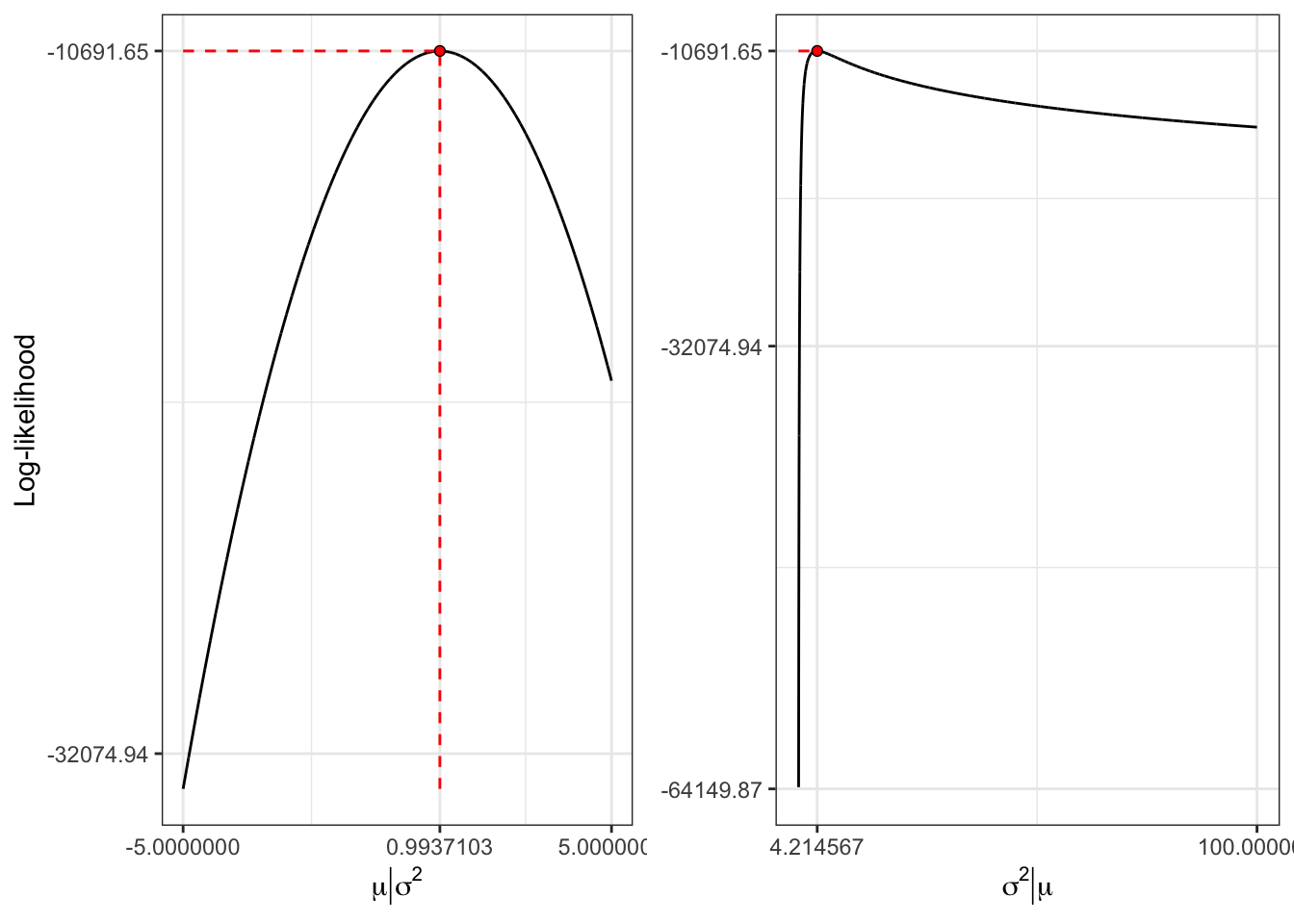
Example 11.1 Let’s simulate 5000 observations from an IID Normal distribution with mean $\mu =1$ and variance ${\sigma }^2=4$. Then, given the simulated sample estimate the maximum likelihood parameters.

library(dplyr)
library(purrr)
################ inputs ################ 
set.seed(1)
n_sim <- 5000 # number of simulations
# true parameters
par <- c(mu = 1, sigma2 = 4)
# normal sample 
x <- rnorm(n_sim, mean = par[1], sd = sqrt(par[2]))
########################################
# log-likelihood for a normal 
loglik_norm <- function(params, x){
  -sum(dnorm(x, mean = params[1], sd = params[2], log = TRUE))
}
# Numerical optimization
opt <- optim(c(0, 1), loglik_norm, x = x)
# best mean parameter 
best_par <- tibble(mu = opt$par[1], sigma = opt$par[2], loglik = -opt$value)

${\mu }^{MLE}$	$\mu$	Mean	$\sigma$	${\sigma }^{MLE}$	Std.deviation
0.994	1	0.994	2	2.053	2.053

Table 11.1: Mean and std. deviation computed on the simulated sample and MLE estimates.

Figure 11.1: Log-likelihood function for a normal sample.

11.2 Quasi-Maximum Likelihood

Quasi-Maximum Likelihood Estimation (QMLE), also known as pseudo-maximum likelihood, is an estimation strategy used when the full distribution may be misspecified but a parametric likelihood can still be posited (e.g., correct conditional mean/variance form, wrong errors). In other words, we assume a parametric likelihood function for the data (perhaps incorrectly) and then maximize it as if it were true.

The QML estimator sacrifices some efficiency (if the model is misspecified there could exists estimators with a lower variance) for for robustness: it converges to the pseudo-true parameter ${\mathit{\theta }}^{\star }$ (the best approximation within the assumed family), and valid inference follows from robust (sandwich) standard errors. This approach yields the quasi-MLE, an estimator that behaves like the true MLE under certain conditions but remains consistent even if the assumed distribution is wrong (See White (1982)).

11.2.1 QML Estimator

Let $f_{{\mathbf{X}}_n}$ be the assumed parametric density function depending on the vector of parameters $\mathit{\theta }$. Then, even if the density $f$ is misspecified, we define the pseudo-true parameter ${\mathit{\theta }}^{\star }$ as the value that maximizes the expected log-likelihood under the true distribution (see Gourieroux, Monfort, and Trognon (1984)), i.e.  $${\mathit{\theta }}^{\star }=\underset{\mathit{\theta }\in \mathrm{\Theta }}{\arg max}\mathbb{E}\{\ell (\mathit{\theta }\mid {\mathbf{X}}_n)\}\text{,}$$ where the expectation is under the true data-generating process. In this case the log-likelihood used is also called pseudo-likelihood because we do not require to work under the true density. Equivalently, ${\mathit{\theta }}^{\star }$ is the value that minimizes the Kullback–Leibler (KL) distance between the true and the (possibly misspecified) parametric density. If the model is correctly specified, ${\mathit{\theta }}^{\star }={\mathit{\theta }}_0$ and QMLE coincides with MLE.

The QML estimator is the sample counterpart and maximize the average log-likelihood given the realized sample ${\mathbf{x}}_n$, i.e.  $${\hat{\mathit{\theta }}}_n^{\text{QML}}=\underset{\mathit{\theta }\in \mathrm{\Theta }}{\arg max}\frac{1}{n}\sum _{i=1}^n\mathcal{L}(\mathit{\theta }\mid x_i)\text{,}$$ Then, to find ${\hat{\mathit{\theta }}}_n^{\text{QML}}$ one proceeds exactly like ordinary MLE optimization finding the vector of parameters that maximizes the average log-likelihood.

11.2.2 Properties

1. Consistency of QMLE: Under the assumption that the model is identifiable at ${\hat{\mathit{\theta }}}_n^{\text{QML}}$, meaning that the expected log-likelihood has a unique maximum at ${\hat{\mathit{\theta }}}_n^{\text{QML}}$ and standard regularity conditions (e.g. continuity of $f(x;\theta )$ in $\theta$) the QMLE estimator converge in probability as $n\to \mathrm{\infty }$ to the pseudo-true parameter, i.e.  $${\hat{\mathit{\theta }}}_n^{\text{QML}}\stackrel{\text{p}}{\underset{n\to \mathrm{\infty }}{⟶}}{\mathit{\theta }}^{\star }\text{.}$$ If the model is correctly specified then the pseudo-true parameter coincides with the actual true parameter, i.e. ${\mathit{\theta }}^{\star }={\mathit{\theta }}_0$, and QMLE reduces to ordinary MLE. However, when the model is misspecified the QMLE parameters converges to ${\mathit{\theta }}^{\star }$ that produces the best approximation of the true distribution, in the sense that it minimize their KL distance.

2. Asymptotic normality: As the MLE, under regularity conditions, the QMLE is asymptotically normal. However, the asymptotic distribution must account for possible misspecification. More precisely, let’s define the expected information computed at the pseudo-true parameter as $$\mathbf{A}({\mathit{\theta }}^{\star })=-\mathbb{E}\{{\mathbf{J}}_{\ell }({\mathit{\theta }}^{\star }\mid {\mathbf{X}}_n)\}$$ and $$\mathbf{B}({\mathit{\theta }}^{\star })=\mathbb{E}\{{\mathrm{\nabla }}_{\ell }({\mathit{\theta }}^{\star }\mid {\mathbf{X}}_n){\mathrm{\nabla }}_{\ell }^{\mathrm{\top }}({\mathit{\theta }}^{\star }\mid {\mathbf{X}}_n)\}$$ Then, a result derived by Huber in the context of M-estimators and White in the context of misspecified likelihoods establishes that under misspecification $\mathbf{A}\ne \mathbf{B}$ and the asymptotic variance is a sandwich of the two matrices, i.e. $$\sqrt{n}({\hat{\mathit{\theta }}}_n^{\text{QML}}-{\mathit{\theta }}^{\star })\stackrel{\text{d}}{\underset{n\to \mathrm{\infty }}{\to }}\text{MVN}(\mathbf{0},{\mathbf{A}}^{-1}({\mathit{\theta }}^{\star })\mathbf{B}({\mathit{\theta }}^{\star }){\mathbf{A}}^{-1}({\mathit{\theta }}^{\star }))\text{,}$$ If the model is correctly specified, then ${\mathit{\theta }}^{\star }={\mathit{\theta }}_0$ and one obtain $$\mathbf{A}({\mathit{\theta }}_0)=-\mathbb{E}\{{\mathbf{J}}_{\ell }({\mathit{\theta }}_0\mid {\mathbf{X}}_n)=\}=\mathbb{E}\{{\mathrm{\nabla }}_{\ell }({\mathit{\theta }}_0\mid {\mathbf{X}}_n){\mathrm{\nabla }}_{\ell }^{\mathrm{\top }}({\mathit{\theta }}_0\mid {\mathbf{X}}_n)\}=\mathbf{B}({\mathit{\theta }}_0)$$ In this case, the the asymptotic variance simplifies and we recover the ML result that is asymptotically efficient. More precisely, the variance covariance matrix of the QMLE $$\mathbb{C}v\{{\hat{\mathit{\theta }}}_n^{\text{QML}}\}=\mathbb{C}v\{{\hat{\mathit{\theta }}}_n^{\text{ML}}\}={\mathbf{A}}^{-1}({\mathit{\theta }}_0)$$ A noteworthy point is that QMLE is generally not fully efficient if the model is misspecified: there might exist other estimators targeting the same quantity that have smaller asymptotic variance if one knew more about the true distribution. But QMLE has the convenience of likelihood-based estimation and retains consistency and asymptotic normality without needing the full truth.

11.2.3 Sandwich Standard Errors

Given the asymptotic variance formula above, a crucial practical issue is how to compute standard errors for QMLE estimates. If one naively computes standard errors as if the assumed model were true (for example, using just the inverse Hessian), the inference can be invalid when the model is misspecified.The remedy is to use robust or sandwich standard errors, often called heteroskedasticity-consistent standard errors in econometrics (See White (1980)).

In practice, to compute the robust variance estimate, one proceeds as follows:

1. First, obtain the QMLE parameters ${\hat{\mathit{\theta }}}_n^{\text{QML}}$ by maximizing the log pseudo log-likelihood.

2. Secondly, compute the average observed Information matrix at the estimated parameter, i.e.  $$\hat{\mathbf{A}}({\hat{\mathit{\theta }}}_n^{\text{QML}})=-\frac{1}{n}\sum _{i=1}^n{\mathbf{J}}_{\ell }({\hat{\mathit{\theta }}}_n^{\text{QML}}\mid {\mathbf{x}}_n)$$

3. Compute the outer product of gradients matrix at the QMLE: $$\hat{\mathbf{B}}({\hat{\mathit{\theta }}}_n^{\text{QML}})=\frac{1}{n}\sum _{t=1}^n{\mathrm{\nabla }}_{\ell }({\hat{\mathit{\theta }}}_n^{\text{QML}}\mid {\mathbf{x}}_n){\mathrm{\nabla }}_{\ell }^{\mathrm{\top }}({\hat{\mathit{\theta }}}_n^{\text{QML}}\mid {\mathbf{x}}_n)$$ This uses the scores for each observation and does not assume the model is correct. Hence, the estimated variance-covariance matrix of the QML parameters reads: $$\mathbb{C}v\{{\hat{\mathit{\theta }}}_n^{\text{QML}}\}=\frac{1}{n}{\hat{\mathbf{A}}}^{-1}({\hat{\mathit{\theta }}}_n^{\text{QML}})\hat{\mathbf{B}}({\hat{\mathit{\theta }}}_n^{\text{QML}}){\hat{\mathbf{A}}}^{-1}({\hat{\mathit{\theta }}}_n^{\text{QML}})$$ where the diagonal elements (scaled by $1/n$) give the variance estimates for each parameter, while the elements outside the diagonal their covariances. Therefore, the variance are obtained as $$\mathbb{V}\{{\hat{\mathit{\theta }}}_n^{\text{QML}}\}=\frac{1}{n}\text{diag}(\mathbb{C}v\{{\hat{\mathit{\theta }}}_n^{\text{QML}}\})$$ if $\hat{\mathbf{A}}$ and $\hat{\mathbf{B}}$ were computed as averages or without rescale if they are summed forms.

If the model is actually correctly specified, then $\hat{\mathbf{B}}$ should be close to $\hat{\mathbf{A}}$ in large samples, and the variance reduces to the usual Fisher information based variance ${\hat{\mathbf{A}}}^{-1}$. Thus, the robust variance estimator is a conservative generalization: it equals the classical one in the ideal case, but remains valid in the non-ideal case.

Gourieroux, Christian, Alain Monfort, and Alain Trognon. 1984. “Pseudo Maximum Likelihood Methods: Theory.” Econometrica 52 (3): 681–700. https://www.jstor.org/stable/1913471.

White, Halbert. 1980. “A Heteroskedasticity-Consistent Covariance Matrix Estimator and a Direct Test for Heteroskedasticity.” Econometrica 48 (4): 817–38. https://doi.org/10.2307/1912934.

———. 1982. “Maximum Likelihood Estimation of Misspecified Models.” Econometrica 50 (1): 1–25. https://doi.org/10.2307/1912526.