9  Introduction

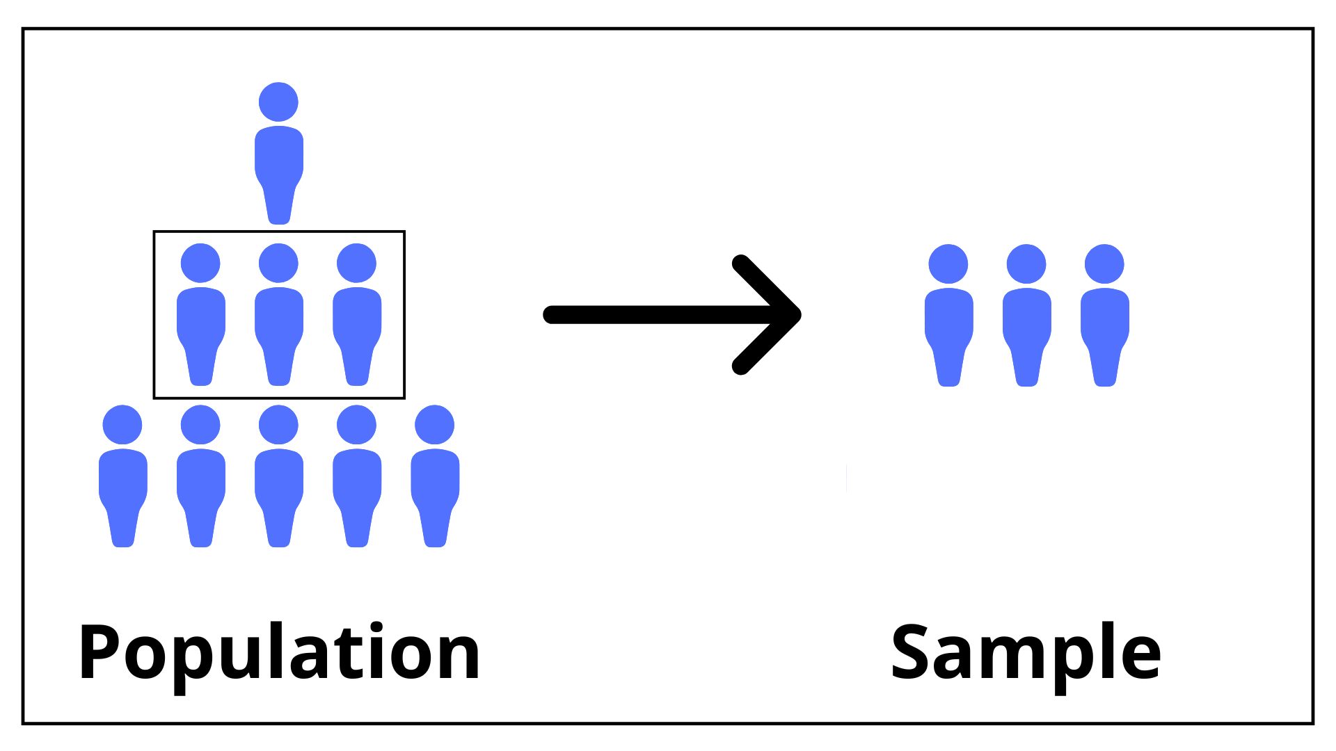
9.1 Population and Sample

A population refers to the entire group of individuals or instances about whom we hope to learn. It encompasses all possible subjects or observations that meet a set of criteria. The population is the complete set of items that interest the researcher, and it can be finite (e.g. the students in a particular school) or infinite (e.g. the number of times a die can be rolled). A population size is given by the number of distinct elements and it includes every individual or observation of interest.

A sample is a subset of the population that is used to represent the population. Since studying an entire population is often impractical due to constraints like time, cost, and accessibility, samples provide a manageable and efficient way to gather data and make inferences about the population. It is important that the sample is representative of the population of interest to allow for valid inferences. It is always important to distinguish between a random sample, e.g. a random group of students in 5th year from a school to make inference about the students at the 5th year of such school, and a convenience sample, e.g. a class of 5th year students who are easily accessible to the researcher, but that can be not representative of all the 5th year students in the school.

Aspect	Population	Sample
Definition	Entire group of interest	Subset of the population
Size	Large, potentially infinite	Small, manageable
Data Collection	Often impractical to study directly	Practical and feasible
Purpose	To understand the whole group	To make inferences about the population

Figure 9.1: Population vs sample.

Population vs sample

Any finite sample is a collection of realization of a finite number of random variables. For example, consider a set of random vector ${\mathbf{X}}_n$, namely a sequence of $n$ random variables ${\mathbf{X}}_n=(X_1,\dots ,X_n)$. Let’s now consider a possible realization of this random sample, namely ${\mathbf{x}}_n=(x_1,\dots ,x_n)$. While ${\mathbf{X}}_n$ denotes a random variable with distributive law given by the joint distribution of $(X_1,\dots ,X_n)$, ${\mathbf{x}}_n$ represents just one of the possible realization of ${\mathbf{X}}_n$.

In general, we distinguish between finite or non-finite populations. In the case of a finite population with $N$ element we distinguish between extractions:

• With reimmission of $n$ elements for the sample gives $N^n$ possible combinations.
• Without readmission of $n$ elements for the sample gives $(\genfrac{}{}{0ex}{}{N}{n})$ possible combinations.

9.2 Estimators

Let’s consider a statistical model depending on some unknown parameter $\theta$ contained in the sample space of parameters $\mathrm{\Theta }$, i.e. $\{P_{\theta }:\theta \in \mathrm{\Theta }\}$. Then, given an observed sample from the statistical model, ${\mathbf{x}}_n=(x_1,\dots ,x_n)$, an estimator is a function that maps the sample space to a set of sample estimates. Formally, since ${\mathbf{X}}_n=(X_1,\dots ,X_n)$ is a collection of random variables, then any function of the sample, like the estimator of $\theta$, is a random variable, i.e.  $${\mathbf{X}}_n⟶{\mathbf{x}}_n⟶\theta ({\mathbf{x}}_n)\text{,}$$ where the random variables in ${\mathbf{X}}_n$ generates a sample ${\mathbf{x}}_n$ that is the input of the estimator function $\theta$ that output an estimate $\theta ({\mathbf{x}}_n)$. When we condition to a particular value of the sample ${\mathbf{x}}_n$, we obtain a point estimate of the true $\theta$, i.e. $\theta ({\mathbf{x}}_n)=\hat{\theta }$, that is a number (or a vector).

Since the estimator is a random variable itself, one can define some metrics to compare different estimators of the same parameter. Firstly, let’s consider the bias, the distance between the average of the collection of estimates and the single parameter being estimated, i.e. $$\mathrm{Bias}\{\theta ({\mathbf{X}}_n)\}=\mathbb{E}\{\theta ({\mathbf{X}}_n)\}-\theta \text{.}$$ We distinguish between two kind of estimators biased, when $$\begin{array}{}\text{(9.1)}& \theta ({\mathbf{X}}_n)\text{biased}⟺\mathrm{Bias}\{\theta ({\mathbf{X}}_n)\}\ne 0\text{,}\end{array}$$ and unbiased, when $$\begin{array}{}\text{(9.2)}& \theta ({\mathbf{X}}_n)\text{unbiased}⟺\mathrm{Bias}\{\theta ({\mathbf{X}}_n)\}=0\text{.}\end{array}$$ The variance is used to indicate how far the collection of estimates are from the expected value of the estimates, i.e. $$\mathbb{V}\{\theta ({\mathbf{X}}_n)\}=\mathbb{E}\left\{{(\theta ({\mathbf{X}}_n)-\mathbb{E}\{\theta ({\mathbf{X}}_n)\})}^2\right\}\text{.}$$ Finally, the Mean Squared Error (MSE) of an estimator, i.e.  $$\mathrm{MSE}\{\theta ({\mathbf{X}}_n)\}=\mathrm{Bias}\{\theta ({\mathbf{X}}_n){\}}^2+\mathbb{V}\{\theta ({\mathbf{X}}_n)\}\text{,}$$ where for an unbiased estimator, the mean squared error equals the variance.

9.2.1 Properties

As for some desirable property of an estimator one have

1. Consistency: An estimator $\theta ({\mathbf{X}}_n)$ is said to be consistent for the parameter $\theta$ if it converges in probability (Definition 8.3) to the true parameter $\theta$ as the sample size $n\to \mathrm{\infty }$: $$\theta ({\mathbf{X}}_n)\underset{n\to \mathrm{\infty }}{\stackrel{\mathbb{P}}{⟶}}\theta \text{.}$$ Intuitively, as the sample grows, the estimator becomes arbitrarily close to the true population’s parameter with high probability, formally for every $\epsilon >0$, $$\underset{n\to \mathrm{\infty }}{lim}\mathbb{P}\{\omega \in \mathrm{\Omega }:|\theta ({\mathbf{X}}_n)-\theta |>ϵ\}=0\text{.}$$ In general, a consistent estimator is a minimal requirement in statistics: without it, the estimator does not converge to the true value even with infinite data. In fact, consistency ensures that the estimator is learning from the data. If we could repeat the estimation process many times with increasing $n$, the histogram of $\hat{\theta }({\mathbf{x}}_n)$ would peak more and more tightly around the true $\theta$. Let’s explore in Example 9.1 the bias and consistency properties of three different estimators of the true expected value of an IID sample.

Example: consistency of an estimator

Example 9.1 Let’s consider an IID normally distributed sample, i.e. $X_1,\dots ,X_n\stackrel{\text{i.i.d.}}{\sim }\mathcal{N}(\mu ,{\sigma }^2)$ and let’s consider different estimators for the mean $\mu$.

A. Sample mean: The natural estimator for $\mu$ under Normality is the sample mean, i.e.  $$\hat{\mu }({\mathbf{x}}_n)=\frac{1}{n}\sum _{i=1}^n{x}_i.$$ that the strong law of large numbers (Proposition 8.1) converges almost surely, and therefore in probability, to the true parameter in population, i.e. $$\hat{\mu }({\mathbf{X}}_n)\stackrel{\text{a.s.}}{⟶}\mu \text{.}$$ Thus $\hat{\mu }$ is a consistent estimator for the true expectation $\mu$. Hence, with more and more samples, the average of the observations will get closer to the true population mean. If we plot $\hat{\mu }$ against $n$, the fluctuations shrink around the true $\mu$.

B. Biased but consistent estimator. Suppose we estimate $\mu$ using an estimator of the form $$\tilde{\mu }({\mathbf{x}}_n)=\frac{1}{n+1}\sum _{i=1}^n{x}_i\text{.}$$ This estimator is biased, since $$\mathbb{E}\{\tilde{\mu }({\mathbf{X}}_n)\}=\frac{n}{n+1}\mu \ne \mu \text{.}$$ However, as $n\to \mathrm{\infty }$, the estimate converges to the true parameter in population, i.e.  $$\underset{n\to \mathrm{\infty }}{lim}\frac{n}{n+1}=1⟹\frac{n}{n+1}\mu \to \mu \text{,}$$ and the variance still shrinks like $1/n$.

Even if ${\tilde{\mu }}_n$ is biased, it can be consistent. Hence, bias does not necessarily prevent consistency if the bias disappears as $n$ grows. In fact, small-sample bias can coexist with asymptotic correctness.

C. Inconsistent estimator: Let’s define as estimator for $\mu$ the value of the first observation, i.e.  $$\underset{―}{\mu }({\mathbf{x}}_n)=x_1\text{.}$$ Clearly, $\underset{―}{\mu }({\mathbf{X}}_n)\sim \mathcal{N}(\mu ,{\sigma }^2)$ for all $n$, so its distribution never concentrates around $\mu$. Formally, $$\mathbb{P}(|\underset{―}{\mu }({\mathbf{X}}_n)-\mu |>\epsilon )=\mathbb{P}(|X_1-\mu |>\epsilon )\ne 0\text{.}$$ Thus, $\underset{―}{\mu }$ is unbiased, but not consistent. Hence, using only one observation, regardless of sample size, ignores the information contained in the data. The variance of the estimator does not reduce with larger $n$.

library(dplyr)
set.seed(1)
# =======================================
#                Inputs 
# =======================================
# True parameters
par <- c(mu = 2, sigma = 2)
# True moments (normal)
moments <- c(par[1], par[2])
# Observations for each sample
n <- c(5, 10, 100, 200, 300, 400, 500)
# Number of samples 
n.sample <- 1000
# Confidence interval 
alpha <- 0.005
# =======================================
# Consistency function 
example_consistency <- function(n = 100, n.sample = 1000, par, moments, alpha = 0.005){
  estimates <- list()
  for(i in 1:n.sample){
    x_n <- rnorm(n, par[1], par[2]) 
    # Case A
    mu_A <- sum(x_n) / n
    # Case B
    mu_B <- mu_A / (n+1) * n
    # Case C
    mu_C <- x_n[1]
    estimates[[i]] <- dplyr::tibble(i = i, n = n,
                                    A = mu_A, 
                                    B = mu_B, 
                                    C = mu_C, 
                                    dw = qnorm(alpha, moments[1], moments[2]/sqrt(n)),
                                    up = qnorm(1-alpha, moments[1], moments[2]/sqrt(n)))
  }
  dplyr::bind_rows(estimates) %>%
  group_by(n) %>%
  mutate(e_A = mean(A), q_dw_A = quantile(A, alpha), q_up_A = quantile(A, 1 - alpha),
         e_B = mean(B), q_dw_B = quantile(B, alpha), q_up_B = quantile(B, 1 - alpha),
         e_C = mean(C), q_dw_C = quantile(C, alpha), q_up_C = quantile(C, 1 - alpha))
}
# =======================================
# Generate data 
data <- purrr::map_df(n, ~example_consistency(.x, n.sample, par, moments, alpha)) 

library(ggplot2)
fig_A <- ggplot(data)+
  geom_point(aes(n, A))+
  geom_line(aes(n, moments[1], color = "theoric"))+
  geom_line(aes(n, e_A, color = "empiric"), linetype = "dashed")+
  geom_line(aes(n, dw, color = "theoric"))+
  geom_line(aes(n, up, color = "theoric"))+
  geom_line(aes(n, q_up_A, color = "empiric"), linetype = "dashed")+
  geom_line(aes(n, q_dw_A, color = "empiric"), linetype = "dashed")+
  theme_bw()+
  scale_color_manual(
    values = c(theoric = "red", empiric = "purple"),
    labels = c(theoric = "Theoric", empiric = "Empiric")
  )+
  theme(legend.position = "none")+
  labs(x = "", y = "", subtitle = "A", color = "")+
  scale_y_continuous(limits = range(c(data$A, data$B, data$C)))

fig_B <- ggplot(data)+
  geom_point(aes(n, B))+
  geom_line(aes(n, moments[1], color = "theoric"))+
  geom_line(aes(n, e_B, color = "empiric"), linetype = "dashed")+
  geom_line(aes(n, dw, color = "theoric"))+
  geom_line(aes(n, up, color = "theoric"))+
  geom_line(aes(n, q_up_B, color = "empiric"), linetype = "dashed")+
  geom_line(aes(n, q_dw_B, color = "empiric"), linetype = "dashed")+
  theme_bw()+
  scale_color_manual(
    values = c(theoric = "red", empiric = "purple"),
    labels = c(theoric = "Theoric", empiric = "Empiric")
  )+
  theme(legend.position = "none")+
  labs(x = "Sample size", y = "", subtitle = "B", color = "")+
  scale_y_continuous(limits = range(c(data$A, data$B, data$C)))

fig_C <- ggplot(data)+
  geom_point(aes(n, C))+
  geom_line(aes(n, moments[1], color = "theoric"))+
  geom_line(aes(n, e_C, color = "empiric"), linetype = "dashed")+
  geom_line(aes(n, dw, color = "theoric"))+
  geom_line(aes(n, up, color = "theoric"))+
  geom_line(aes(n, q_up_C, color = "empiric"), linetype = "dashed")+
  geom_line(aes(n, q_dw_C, color = "empiric"), linetype = "dashed")+
  theme_bw()+
  scale_color_manual(
    values = c(theoric = "red", empiric = "purple"),
    labels = c(theoric = "Theoric", empiric = "Empiric")
  )+
  theme(legend.position = "none")+
  labs(x = "", y = "", subtitle = "C", color = "")+
  scale_y_continuous(limits = range(c(data$A, data$B, data$C)))

gridExtra::grid.arrange(fig_A, fig_B, fig_C, nrow = 1)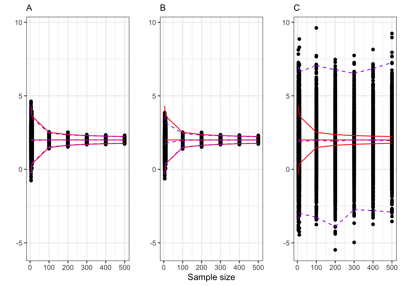

Sample means computed on 1000 samples with different number of observations with estimators A, B and C. The theoric confidence interval and true expectation of $\mu$ in red while in purple the empirical ones.

2. Efficiency: Among unbiased estimators, the one with minimal variance is called efficient; asymptotically efficient means it attains the Cramér–Rao lower bound (CRLB) limit.

3. Asymptotic normality: for some normalizing sequence $a_n$ depending on $n$, the estimator converges in distribution (Definition 8.5) to a normal random variable, $$a_n(\theta ({\mathbf{X}}_n)-\theta )\underset{n\to \mathrm{\infty }}{\stackrel{\text{d}}{⟶}}\mathcal{N}(0,{\sigma }^2(\theta ))\text{.}$$

9.2.2 Sufficiency and Completeness

Theorem 9.1 ($\mathbf{\text{Factorization Theorem}}$)
A statistic $\theta ({\mathbf{X}}_n)$ is sufficient for the parameter $\theta$ if and only if the joint density (or probability mass function) can be factorized as $$f({\mathbf{X}}_n\mid \theta )=g(\theta ({\mathbf{X}}_n),\theta )h({\mathbf{X}}_n)\text{,}$$ for some non-negative functions $g$ and $h$, where $g$ depends on the data only through $\theta ({\mathbf{X}}_n)$ and $\theta$, while $h$ does not depend on the parameter $\theta$.

In other words, a statistic is sufficient if it captures all the information in the sample about $\theta$. After observing a sufficient statistic, the sample provides no further information about the parameter $\theta$. Equivalently, the conditional distribution of the full data given the sufficient statistic does not depend on $\theta$. A natural consequence of sufficiency is that two samples with the same value for the sufficient statistic should result in the same inference.

Example: Sufficient statistic for a Bernoulli

Example 9.2 If ${\mathbf{X}}_n\stackrel{\text{iid}}{\sim }\text{Bernoulli}(p)$, the likelihood given $p$ is $$f({\mathbf{X}}_n\mid p)=p^{\sum _{i=1}^n{X}_i}(1-p{)}^{n-\sum _{i=1}^n{X}_i}\text{.}$$ Here $K({\mathbf{X}}_n)=\sum _{i=1}^n{X}_i$ is sufficient for $p$, since the likelihood factors as $g(K,p)=p^K(1-p{)}^{n-K}$ with $h({\mathbf{X}}_n)=1$. Intuitively: for Bernoulli trials, only the total number of successes matters, not the specific order.

Theorem 9.2 ($\mathbf{\text{Rao–Blackwell}}$)
If $\theta ({\mathbf{X}}_n)$ is sufficient for $\theta$ and ${\theta }^{\prime }({\mathbf{X}}_n)$ is any unbiased estimator of $\theta$, then the Rao–Blackwellized estimator $$\begin{array}{}\text{(9.3)}& {\theta }^{RB}({\mathbf{X}}_n)=\mathbb{E}\{{\theta }^{\prime }({\mathbf{X}}_n)\mid \theta ({\mathbf{X}}_n)\}\text{,}\end{array}$$ is unbiased for $\theta$, i.e. $\mathbb{E}\{{\theta }^{RB}({\mathbf{X}}_n)\}=\theta$ and has a lower (or equal) variance than ${\theta }^{\prime }$ $$\mathbb{V}\{{\theta }^{RB}({\mathbf{X}}_n)\}\le \mathbb{V}\{{\theta }^{\prime }({\mathbf{X}}_n)\}\text{.}$$

In other words, conditioning on a sufficient statistic cannot increase variance. So Rao–Blackwell gives a systematic way to improve an estimator: start with any unbiased estimator, then condition it on a sufficient statistic to possibly reduced the variance.

Definition 9.1 ($\mathbf{\text{Completeness}}$)
A statistic $\theta ({\mathbf{X}}_n)$ is said to be complete if for any measurable function $g$ and for all $\theta \in \mathrm{\Theta }$, $$\mathbb{E}\{g(\theta ({\mathbf{X}}_n))\mid \theta \}=0\text{,}$$ implies that $$g(\theta ({\mathbf{X}}_n))=0\text{,}$$ almost surely (Definition 8.2).

Intuition: if a function of a statistic always averages out to zero no matter what the parameter is, then it must be the trivial zero function. Completeness rules out the existence of “hidden functions” of the statistic that are unbiased estimators of $\theta$ but nontrivial. It ensures uniqueness of unbiased estimators derived from the statistic.

Example: Complete and sufficient statistic for a Bernoulli

Example 9.3 Continuing from Example 9.2, the statistic $K({\mathbf{X}}_n)=\sum _{i=1}^n{X}_i$ is not only sufficient but also complete for $p$. In fact if a function $g$ satisfies $\mathbb{E}\{g(K({\mathbf{X}}_n))\}=0$ for all $p$, then necessarily $g(.)=0$. Suppose there exists some function g such that for all $p\in (0,1)$ $$\mathbb{E}\{g(T)\}=\sum _{t=0}^{n}g(t)(\genfrac{}{}{0ex}{}{n}{t})p^t(1-p{)}^{n-t}=0\text{.}$$ The left-hand side is a polynomial in $p$ (because of the binomial expansion). If this polynomial is identically zero for all $p$, then all coefficients must be zero and so each $g(t)=0$.

Theorem 9.3 ($\mathbf{\text{Lehmann–Scheffé Theorem}}$)
If $\theta ({\mathbf{X}}_n)$ is complete and sufficient estimator of $\theta$, and if ${\theta }^{RB}({\mathbf{X}}_n)$, as defined in Equation 9.3, is unbiased for $\theta$, then ${\theta }^{RB}({\mathbf{X}}_n)$ is the unique Uniformly Minimum-Variance Unbiased Estimator (UMVU) of $\theta$.

In practice, sufficiency (Theorem 9.1) ensures ${\theta }^{RB}({\mathbf{X}}_n)$ uses all available information and completeness (Definition 9.1) ensures no other unbiased estimator can have the same mean with smaller variance. Thus, the Lehmann–Scheffé theorem identifies the best possible unbiased estimator.

Example: UMVU estimator of $p$ for a Bernoulli

Example 9.4 Continuing from Example 9.3, $K({\mathbf{X}}_n)=\sum _{i=1}^n{X}_i$ is complete and sufficient for $p$. Thus, by Lehmann–Scheffé, the sample mean is an unbiased UMVU estimator of $p$.