3  Measurable maps

Reference: Chapter 3. Resnick (2005).

A measurable space is composed by a sample space $\mathrm{\Omega }$ and a $\sigma$-field of subsets of $\mathrm{\Omega }$, namely $\mathcal{B}$.

3.1 Maps and inverse maps

Let’s be very general and consider two measurable spaces $(\mathrm{\Omega },\mathcal{B})$, $({\mathrm{\Omega }}^{\prime },{\mathcal{B}}^{\prime })$ and a map (function) $X(\omega )$ that associate to every $\omega \in \mathrm{\Omega }$ an outcome ${\omega }^{\prime }\in {\mathrm{\Omega }}^{\prime }$, i.e.  $$X:(\mathrm{\Omega },\mathcal{B})\to ({\mathrm{\Omega }}^{\prime },{\mathcal{B}}^{\prime })\text{.}$$ Then, $X$ determine a function $X^{-1}$ called inverse map, i.e.  $$X^{-1}:\mathcal{P}({\mathrm{\Omega }}^{\prime })\to \mathcal{P}(\mathrm{\Omega })\text{.}$$ where $\mathcal{P}$ denotes the power set, i.e. the set of all subsets and the largest $\sigma$-field available. Then, $X^{-1}$ is defined such that for every set $B^{\prime }$ in ${\mathrm{\Omega }}^{\prime }$ $$\begin{array}{}\text{(3.1)}& X^{-1}(B^{\prime })=\{\omega \in \mathrm{\Omega }:X(\omega )\in B^{\prime }\}\text{.}\end{array}$$

Exercise 3.1 Let’s consider a deck of poker cards with 52 cards in total. We have 4 groups of 13 distinct cards, where the Jack (J) is 11, the Queen (Q) is 12, the King (K) is 13 and Ace (A) is 14. Then, let’s consider function of the form $$X(\omega )=\{\begin{array}{l}+1\text{if}\omega \in \{2,3,4,5,6\}\\ 0\text{if}\omega \in \{7,8,9\}\\ -1\text{if}\omega \in \{10,11,12,13,14\}\end{array}$$ In this case the sample space $\mathrm{\Omega }$ is composed by 14 unique elements (52 elements in total, i.e. all the cards), while ${\mathrm{\Omega }}^{\prime }=\{-1,0,1\}$ represents the possible outcomes. Let’s say that one observe a value $X(\omega )=\{+1\}\subset {\mathrm{\Omega }}^{\prime }$, define $X^{-1}(\{+1\})$ according to Equation 3.1.

Solution: Exercise 3.1

Solution 3.1. Let’s say that one observe a value $X(\omega )=\{+1\}\subset {\mathrm{\Omega }}^{\prime }$, then the inverse map $X^{-1}$ identifies the set of $\omega$ such that $X(\omega )=\{+1\}$, i.e.  $$X^{-1}(\{+1\})=\{\omega \in \mathrm{\Omega }:X(\omega )\in \{+1\}\}=\{2,3,4,5,6\}\text{.}$$

The inverse map $X^{-1}$ has many properties. Among them, it preserves complementation, union and intersection.

1. $X^{-1}({\mathrm{\Omega }}^{\prime })=\mathrm{\Omega }$.
2. $X^{-1}(\mathrm{\varnothing })=\mathrm{\varnothing }$.
3. $X^{-1}(A^{\prime \mathsf{c}})=(X^{-1}(A^{\prime }){)}^{\mathsf{c}}$.
4. $X^{-1}({\mathrm{\Omega }}^{\prime }\cap A^{\prime })=\mathrm{\Omega }\cap X^{-1}(A^{\prime \mathsf{c}})$.
5. $X^{-1}(\bigcup _n{A}_n^{\prime })=\bigcup _n{X}^{-1}(A_n^{\prime })$ for all $A_n^{\prime }\in {\mathcal{B}}^{\prime }$.

Properties of inverse maps

Let’s consider two sets $A^{\prime }$ and $B^{\prime }$ both in ${\mathrm{\Omega }}^{\prime }$. Then, by definition: $$\begin{array}{rl}{X}^{-1}(A^{\prime }\cup B^{\prime })& =\{\omega \in \mathrm{\Omega }:X(\omega )\in A^{\prime }\cup B^{\prime }\}=\\ & =\{\omega \in \mathrm{\Omega }:X(\omega )\in A^{\prime }\text{OR}X(\omega )\in B^{\prime }\}=\\ & =\{\omega \in \mathrm{\Omega }:X(\omega )\in A^{\prime }\}\cup \{\omega \in \mathrm{\Omega }:X(\omega )\in B^{\prime }\}=\\ & =X^{-1}(A^{\prime })\cup X^{-1}(B^{\prime })\end{array}$$ Similarly for the intersection, i.e.  $$\begin{array}{rl}{X}^{-1}(A^{\prime }\cap B^{\prime })& =\{\omega \in \mathrm{\Omega }:X(\omega )\in A^{\prime }\cap B^{\prime }\}=\\ & =\{\omega \in \mathrm{\Omega }:X(\omega )\in A^{\prime }\text{AND}X(\omega )\in B^{\prime }\}=\\ & =\{\omega \in \mathrm{\Omega }:X(\omega )\in A^{\prime }\}\cap \{\omega \in \mathrm{\Omega }:X(\omega )\in B^{\prime }\}=\\ & =X^{-1}(A^{\prime })\cap X^{-1}(B^{\prime })\end{array}$$

Proposition 3.1 If ${\mathcal{B}}^{\prime }$ is a $\sigma$-field of subsets of ${\mathrm{\Omega }}^{\prime }$, then $X^{-1}({\mathcal{B}}^{\prime })$ is a $\sigma$-field of subsets of $\mathrm{\Omega }$. Moreover, if ${\mathcal{C}}^{\prime }$ is a class of subsets of ${\mathrm{\Omega }}^{\prime }$, then $$X^{-1}(\sigma (C^{\prime }))=\sigma (X^{-1}(C^{\prime }))\text{,}$$ that is. the inverse image of the $\sigma$-field generated by the class ${\mathcal{C}}^{\prime }\in {\mathrm{\Omega }}^{\prime }$ is the same as the $\sigma$-field generated in $\mathrm{\Omega }$ by the inverse image $X^{-1}$. In practice, the counter image and the generators commute. Usually can be difficult to know all about the $\sigma$-field ${\mathcal{B}}^{\prime }$, however if we know a class of subset that generate it, namely ${\mathcal{C}}^{\prime }\in {\mathrm{\Omega }}^{\prime }$, we are able to recreate the $\sigma$-field. (References: propositions 3.1.1, 3.1.2. A prob path).

3.1.1 Measurable maps

Definition 3.1 ($\mathbf{\text{Measurable map}}$)
Let’s consider the function $X:(\mathrm{\Omega },\mathcal{B})\to ({\mathrm{\Omega }}^{\prime },{\mathcal{B}}^{\prime })$, then $X$ is $\mathcal{B}$-measurable, namely $X\in \mathcal{B}/{\mathcal{B}}^{\prime }$, iff: $$X\in \mathcal{B}/{\mathcal{B}}^{\prime }⟺X^{-1}({\mathcal{B}}^{\prime })\in \mathcal{B}\text{.}$$

Note that the measurability concept is very important since only if $X$ is measurable it is possible to make probability statements about $X$. In fact, the probability is nothing more than a type of measure, only if $X^{-1}(B^{\prime })\in \mathcal{B}$ for all $B^{\prime }\in {\mathcal{B}}^{\prime }$ it is possible to assign a measure (probability) to the events that are contained in $\mathcal{B}$.

Definition 3.2 ($\mathbf{\text{Test for measurability}}$)
Consider a map $X:(\mathrm{\Omega },\mathcal{B})\to ({\mathrm{\Omega }}^{\prime },{\mathcal{B}}^{\prime })$ and the class ${\mathcal{C}}^{\prime }$ that generates the $\sigma$-field ${\mathcal{B}}^{\prime }$, i.e. ${\mathcal{B}}^{\prime }=\sigma ({\mathcal{C}}^{\prime })$. Then $X$ is $\mathcal{B}$-measurable iff: $$X\in \mathcal{B}/{\mathcal{B}}^{\prime }⟺X^{-1}({\mathcal{C}}^{\prime })\subset \mathcal{B}\text{.}$$

3.2 Random variables

Definition 3.3 ($\mathbf{\text{Random variable}}$)
Let’s consider a probability space $(\mathrm{\Omega },\mathcal{F},\mathbb{P})$, then a random variable is a map (function) where $({\mathrm{\Omega }}^{\prime },{\mathcal{B}}^{\prime })=(\mathbb{R},\mathcal{B}(\mathbb{R}))$. Therefore it takes values on the real line, i.e. $$X:(\mathrm{\Omega },\mathcal{B})\to (\mathbb{R},\mathcal{B}(\mathbb{R}))$$ and for every set $B$ in the Borel $\sigma$-field generated by the real line $\mathcal{B}(\mathbb{R})$, the counter image of $B$, namely $X^{-1}(B)$ is in the $\sigma$-field $\mathcal{B}$ generated by $\mathrm{\Omega }$. Formally, $$\mathrm{\forall }B\in \mathcal{B}(\mathbb{R})X^{-1}(B)=\{\omega \in \mathrm{\Omega }:X(\omega )\in B\}\subset \mathcal{B}\text{.}$$ More precisely, when $X$ is a random variable the test for measurability (Definition 3.2), became: $$X^{-1}((-\mathrm{\infty },y])=[X(\omega )\le y]\subset \mathcal{B}\mathrm{\forall }y\in \mathbb{R}\text{.}$$ In practice, $B=(-\mathrm{\infty },y]$ that depends on the real number $y$ while the event $[X(\omega )\le y]=X^{-1}(B)$ is exactly the counter image of $B$.

3.2.1 $\sigma$-field generated by a map

Let $X:(\mathrm{\Omega },\mathcal{B})\to ({\mathrm{\Omega }}^{\prime },{\mathcal{B}}^{\prime })$ be a measurable map, then the $\sigma$-field generated by $X$ is defined as: $$\sigma (X)=X^{-1}({\mathcal{B}}^{\prime })=\{\omega \in \mathrm{\Omega }:X(\omega )\in B^{\prime },B^{\prime }\in {\mathcal{B}}^{\prime }\}$$ When $X$ is a random variable, then $({\mathrm{\Omega }}^{\prime },{\mathcal{B}}^{\prime })=(\mathbb{R},\mathcal{B}(\mathbb{R}))$ and the $\sigma$-field generated by $X$ $$\sigma (X)=X^{-1}(\mathcal{B}(\mathbb{R}))=\{\omega \in \mathrm{\Omega }:X(\omega )\in B,B\in \mathcal{B}(\mathbb{R})\}$$

Definition 3.4 Let $X$ be a random variable with set of possible outcomes ${\mathrm{\Omega }}^{\prime }$. Then, $X$ is called

• discrete random variable if ${\mathrm{\Omega }}^{\prime }$ is either a finite set or a countably infinite set.
• continuous random variable if ${\mathrm{\Omega }}^{\prime }$ is either a an uncountable infinite set.

Definition 3.5 A random vector is a map $${\mathbf{X}}_n:(\mathrm{\Omega },\mathcal{B})\to ({\mathbb{R}}^n,\mathcal{B}({\mathbb{R}}^n))$$ It’s counter image ${\mathbf{X}}^{-1}$ is defined as: $$\mathrm{\forall }B\in \mathcal{B}({\mathbb{R}}^n){\mathbf{X}}_n^{-1}(B)=\{\omega \in \mathrm{\Omega }:{\mathbf{X}}_n(\omega )\in B\}\in \mathcal{B}$$ Note that, for every $\omega$, the random vector has $n$-components, i.e.  $${\mathbf{X}}_n(\omega )=\left(\begin{array}{c}{X}_1(\omega )\\ X_2(\omega )\\ ⋮\\ X_n(\omega )\end{array}\right)$$

Proposition 3.2 The map ${\mathbf{X}}_n:(\mathrm{\Omega },\mathcal{B})\to ({\mathbb{R}}^n,\mathcal{B}({\mathbb{R}}^n))$ is a random vector, if and only if each component $X_1,X_2,\dots ,X_n$ is a random variable.

Proof: Proposition 3.2

Proof. Let’s prove that if $X_1,X_2,\dots ,X_n$ are random variables, then $\underset{―}{\mathbf{X}}$ is a random vector. Since we are assuming that each $i$-th component is a random variable we have that for all $i=1,2,\dots ,n$ $$\mathrm{\forall }{y}_i\in \mathbb{R}{X}_i^{-1}((-\mathrm{\infty },y_i])\in \mathcal{B}\text{.}$$ Therefore, to prove that ${\mathbf{X}}_n$ is a random vector we have to prove that the cartesian product of all the counter images, i.e.  $$\{\omega \in \mathrm{\Omega }:X_1\in (\mathrm{\infty },y_1]\cap X_2\in (\mathrm{\infty },y_2]\cap \cdots \cap X_k\in (\mathrm{\infty },y_k]\}\text{,}$$ is in $\mathcal{B}$. That is equivalent to the intersection $$\bigcap _{i=1}^k\{\omega \in \mathrm{\Omega }:X_i\in (\mathrm{\infty },y_i]\}=\bigcap _{i=1}^k{X}_i^{-1}((\mathrm{\infty },y_i])\in \mathcal{B}\text{.}$$ Since, each the counter image of each $X_i^{-1}((\mathrm{\infty },y_i])\in \mathcal{B}$ and $\mathcal{B}$ is a $\sigma$-field, hence closed under countable intersection, also the intersection of all the counter images will be in $\mathcal{B}$.

3.3 Induced distribution function

Consider a probability space $(\mathrm{\Omega },\mathcal{B},\mathbb{P})$ and a measurable map $X:(\mathrm{\Omega },\mathcal{B})\to ({\mathrm{\Omega }}^{\prime },{\mathcal{B}}^{\prime })$, then the composition $\mathbb{P}\circ X^{-1}$ is again a map. In this way at each element $\omega \in \mathrm{\Omega }$ is attached a probability measure. In fact, the composition is a map such that $$\mathbb{P}\circ X^{-1}:({\mathrm{\Omega }}^{\prime },{\mathcal{B}}^{\prime })\to [0,1]⟺({\mathrm{\Omega }}^{\prime },{\mathcal{B}}^{\prime })\stackrel{X^{-1}}{⟶}(\mathrm{\Omega },\mathcal{B})\stackrel{\mathbb{P}}{⟶}[0,1]$$ In general, the probability of a subset $A^{\prime }\in {\mathcal{B}}^{\prime }$ is denoted equivalently as: $$\mathbb{P}\circ X^{-1}(A^{\prime })=\mathbb{P}(X^{-1}(A^{\prime }))=\mathbb{P}(X(\omega )\in A^{\prime })$$

Exercise 3.2 Let’s continue from the Exercise 3.1 and compute the probability of $\mathbb{P}\circ X^{-1}(\{+1\})$. Let’s consider one random extraction from the 52 cards, then for each distinct number we have 4 copies. Compute $\mathbb{P}(X^{-1}(\{+1\}))$ and $\mathbb{P}(X^{-1}(\{0\}))$.

Solution: Exercise 3.2

Solution 3.2. The probability is computed as: $$\begin{array}{rl}\mathbb{P}(X^{-1}(\{+1\}))& =\mathbb{P}(\{\omega \in \mathrm{\Omega }:X(\omega )\in \{-1\}\})=\\ & =\mathbb{P}(\{2,3,4,5,6\})=\\ & =\frac{5\cdot 4}{52}=\frac{5}{13}\approx 38.46\mathrm{\%}\end{array}$$ Let’s consider the probability of observing either $\{+1\}$ or $\{-1\}$, then $$\begin{array}{rl}\mathbb{P}(X^{-1}(\{-1,+1\}))& =\mathbb{P}(\{\omega \in \mathrm{\Omega }:X(\omega )\in \{-1,+1\}\})=\\ & =\mathbb{P}(\{2,3,4,5,6,10,11,12,13,14\})=\\ & =\frac{10\cdot 4}{52}=\frac{10}{13}\approx 76.92\mathrm{\%}\end{array}$$ Finally, by property of the probability measure $\mathbb{P}(X(\omega )\in \{0\})=1-\mathbb{P}(X(\omega )\in \{-1,+1\})\approx 23.08\mathrm{\%}$.

3.3.1 Distribution function on $\mathbb{R}$

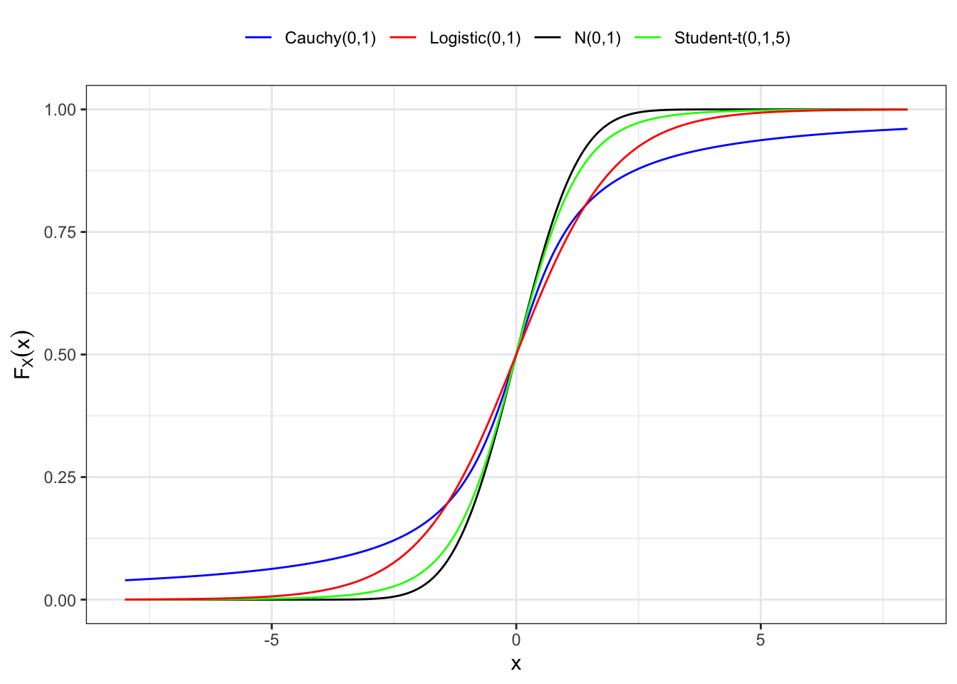
When $X$ is a random variable the composition $\mathbb{P}(X^{-1}(A^{\prime }))$ is a probability measure induced on $\mathbb{R}$ by the composition: $$\mathbb{P}(X^{-1}((-\mathrm{\infty },y])=\mathbb{P}(X\le y)=F_X(y)\text{,}$$ for all $y$ in $\mathbb{R}$. Hence, the distribution function $F_X$ of a random variable $X$ is a function $F_X:(\mathbb{R},\mathcal{B}(\mathbb{R}))\to [0,1]$ and represents a probability measure on the real line $\mathbb{R}$, i.e.  $$F_X(y)=\mathbb{P}(X(\omega )\in [-\mathrm{\infty },y))=\mathbb{P}(X(\omega )\le y)\text{,}$$ or for short $\mathbb{P}(X\le y)$.

Warning

In general, the probability distribution is a function $F_X:({\mathrm{\Omega }}^{\prime },{\mathcal{B}}^{\prime })\to [0,1]$, however when $X$ is a random variable this means that $({\mathrm{\Omega }}^{\prime },{\mathcal{B}}^{\prime })=(\mathbb{R},\mathcal{B}(\mathbb{R}))$.

(a) Distribution functions.

(b) Quantile functions.

Figure 3.1: Different distribution functions in $\mathbb{R}$.

Proposition 3.3 ($\mathbf{\text{Density of a random variable}}$)
If a random variable $X$ has a continuous and differentiable distribution function, then its probability density function (pdf) is defined as the first derivative of the distribution function with respect to $y$, i.e. $$\begin{array}{}\text{(3.2)}& f_X(y)=\frac{d}{dy}{F}_X(y)⟺d{F}_X(y)=f_X(y)dy\text{.}\end{array}$$ Instead, for a discrete random variable we call it probability mass function (pmf), i.e.  $$f_X(y)=\mathbb{P}(X=y)\text{.}$$ Considering a generic domain $\mathcal{D}\subseteq \mathbb{R}$ for the random variable $X$, then the function $f_X$ satisfies two fundamental properties, i.e.

1. Positivity: $f_X(y)\ge 0$ for all $y\in \mathcal{D}$.
2. Normalization: ${\int }_{\mathcal{D}}{f}_X(y)dy=1$ or $\sum _{y\in \mathcal{D}}\mathbb{P}(X=y)=1$.

Warning

In general, any function $f_X$ that satisfies properties 1. and 2. in Proposition 3.3 is the density function of some (unknown) random variable.

3.3.2 Survival function

For any random variable with distribution $F_X$, the survival distribution is defined as: $${\overline{F}}_X(y)=\mathbb{P}(X\ge y)=1-F_X(y)\text{.}$$

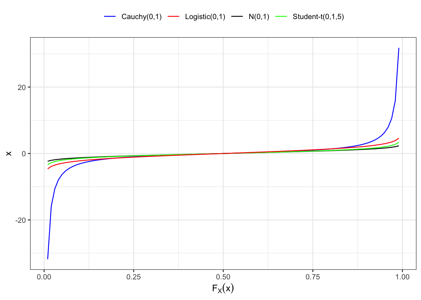
Definition 3.6 ($\mathbf{\text{Criterion I for heavy tails}}$)
A distribution function $F_X$ is said to be:

1. Light tailed if for some $\lambda >0$ $$\underset{y\to \mathrm{\infty }}{lim}\frac{{\overline{F}}_X(y)}{e^{-\lambda y}}=\{\begin{array}{ll}0& \text{faster than exponential}\\ 0<l<\mathrm{\infty }& \text{same speed as the exponential}\end{array}$$

2. Heavy tailed if for all $\lambda >0$ $$\underset{y\to \mathrm{\infty }}{lim}\frac{{\overline{F}}_X(y)}{e^{-\lambda y}}=\mathrm{\infty }\text{slower than the exponential}\text{.}$$

Resnick, Sidney I. 2005. A Probability Path. Birkhauser. https://link.springer.com/book/10.1007/978-0-8176-8409-9.