1 Basic set theory
Reference: Chapter 1. Resnick (2005).
In probability, an event is interpreted as a collection of possible outcomes of a random experiment.
Definition 1.1 (Random experiment) A random experiment is any repeatable procedure that results in one out of a well-defined set of possible outcomes.
- The set of possible outcomes is called the sample space and denoted by \(\Omega\). An element of \(\Omega\) is denoted by \(\omega\) and is an outcome
- A set of zero or more outcomes \(\omega\) is an event \(A\), where we denote a class of subsets \(A \subset \Omega\) by \(\mathcal{F}\).
- A map (function) that goes from the space of the events \(\mathcal{F}\) to the space of probabilities (real numbers in \([0, 1]\)) is the probability law and is denoted with \(\mathbb{P}\).
Together, sample space, event space and probability law characterize a random experiment.
There are several definitions related to sets and their operations.
Definition 1.2 (Complementation) The complement of a set \(A\) is denoted by \(A^{\mathsf{c}}\) and represents the set of elements that do not belong to \(A\), i.e. \[ A^{\mathsf{c}} = \{\omega \in \Omega : \omega \not\in A\} \text{.} \tag{1.1}\]
Definition 1.3 (Containment) A set \(A\) is said to be contained in a set \(B\) if every element of \(A\) is also an element of \(B\). Formally, \[ A \subset B \iff \omega \in A \implies \omega \in B \quad \forall \omega \in \Omega \text{.} \tag{1.2}\]
Definition 1.4 (Equality) Given two sets, \(A\) is equal to \(B\), written \(A = B\), if and only if every element of \(A\) is an element of \(B\) and every element of \(B\) is an element of \(A\). Formally, \[ A \subset B \quad\text{and}\quad B \subset A \text{.} \tag{1.3}\]
1.1 Set operations
Let’s now state some elementary operations between sets.
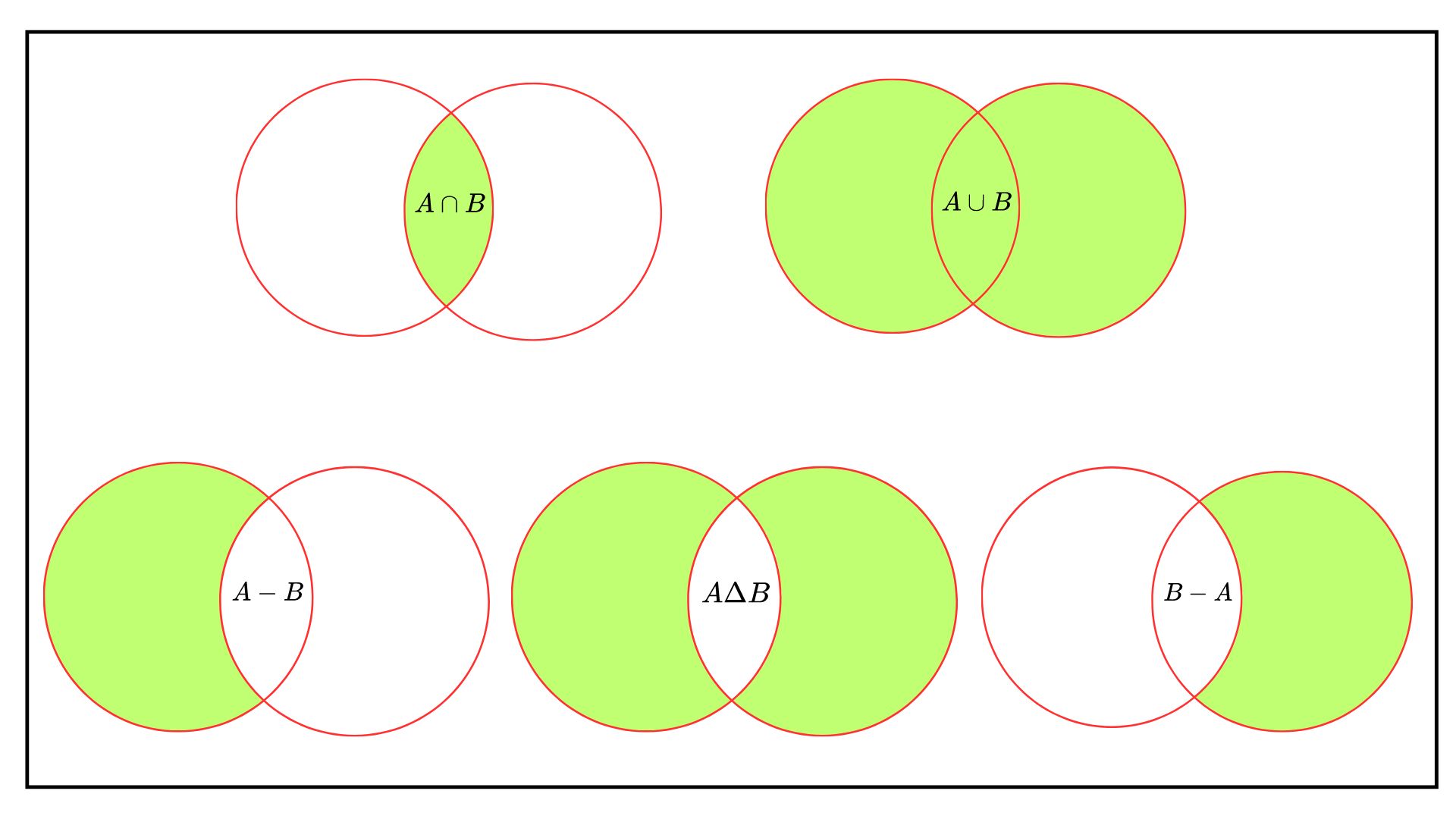
Definition 1.5 (Union) The union of two sets, written \(A {\color{red}{\cup}} B\), is the set of \(\omega\) that belong either to \(A\) or to \(B\), i.e. \[ A {\color{red}{\cup}} B = \{\omega \in \Omega : \omega \in A \text{ or } \omega \in B\} \text{.} \tag{1.4}\]
As a consequence of the definition of the union, the following relations hold true, i.e. \[ \begin{aligned} & {} A {\color{red}{\cup}} A = A && {} A {\color{red}{\cup}} \Omega = \Omega \\ & A {\color{red}{\cup}} \emptyset = A && A {\color{red}{\sqcup}} A^{\mathsf{c}} = \Omega \end{aligned} \]
Definition 1.6 (Intersection) The intersection of \(A\) and \(B\) is written \(A {\color{blue}{\cap}} B\) and is the set of elements that belong at the same time to \(A\) and \(B\). \[ A {\color{blue}{\cap}} B = \{\omega \in \Omega: \omega \in A \text{ and } \omega \in B\} \text{.} \]
As a consequence of the definition of the intersection, the following relations hold, i.e. \[ \begin{aligned} & {} A {\color{blue}{\cap}} A = A && {} A {\color{blue}{\cap}} \Omega = A \\ & A {\color{blue}{\cap}} \emptyset = \emptyset && A {\color{blue}{\sqcap}} A^{\mathsf{c}} = \emptyset \end{aligned} \] Moreover, let’s state the distributive laws of the union and the intersection, i.e. \[ \begin{aligned} & {} \mathbf{Intersection}.\quad && {} (A {\color{red}{\cup}} B) {\color{blue}{\cap}} C = (A {\color{blue}{\cap}} C) {\color{red}{\cup}} (B {\color{blue}{\cap}} C) \\ & \mathbf{Union}.\quad && (A {\color{blue}{\cap}} B) {\color{red}{\cup}} C = (A {\color{red}{\cup}} C) {\color{blue}{\cap}} (B {\color{red}{\cup}} C) \end{aligned} \tag{1.5}\] And the De Morgan’s laws: \[ \begin{aligned} & {} \mathbf{Intersection}.\quad && {} (A {\color{blue}{\cap}} B)^{\mathsf{c}} = (A^{\mathsf{c}} {\color{red}{\cup}} B^{\mathsf{c}}) \\ & \mathbf{Union}.\quad && (A {\color{red}{\cup}} B)^{\mathsf{c}} = (A^{\mathsf{c}} {\color{blue}{\cap}} B^{\mathsf{c}}) \end{aligned} \tag{1.6}\]
Definition 1.7 (Difference) The difference between two sets \(A\) and \(B\), written \(A-B\) (or also \(A / B\)), is the set of elements of \(A\) that do not belong to \(B\). Formally \[ A-B = A {\color{blue}{\cap}} B^{\mathsf{c}} = \{\omega \in \Omega : \omega \in A \text{ and } \omega \not\in B\} \text{.} \tag{1.7}\]
Disjoint representation of a set
Given two sets \(A\) and \(B\), each one can be written as the union of disjoint sets. In fact, their union can be decomposed into the union of three disjoint sets, i.e. \[ A {\color{red}{\sqcup}} B = (A {\color{blue}{\cap}} B) {\color{red}{\sqcup}} (A {\color{blue}{\cap}} B^{\mathsf{c}}) {\color{red}{\sqcup}} (A^{\mathsf{c}} {\color{blue}{\cap}} B) \text{,} \tag{1.8}\] and therefore for example the set \(A\) can be written as \[ A = (A {\color{blue}{\cap}} B) {\color{red}{\sqcup}} (A - B) = (A {\color{blue}{\cap}} B) {\color{red}{\sqcup}} (A {\color{blue}{\cap}} B^{\mathsf{c}}) \text{.} \tag{1.9}\]
Definition 1.8 (Symmetric difference) The symmetric difference between two sets \(A\) and \(B\) is written \(A \Delta B\) and is the union of elements of \(A\) that do not belong to \(B\) and of elements of \(B\) that do not belong to \(A\), i.e. \[ \begin{aligned} A \Delta B & {} = (A - B) {\color{red}{\sqcup}} (B - A) = \\ & = (A {\color{blue}{\cap}} B^{\mathsf{c}}) {\color{red}{\sqcup}} (A^{\mathsf{c}} {\color{blue}{\cap}} B) = \\ & = \{\omega : \omega \in A, \, \omega \not\in B \} {\color{red}{\sqcup}} \{\omega : \omega \in B,\, \omega \not\in A \} \end{aligned} \]
Proposition 1.1 Given two sets \(A,B\), the symmetric difference can be written as \[ A \Delta B = (A {\color{red}{\sqcup}} B) {\color{blue}{\cap}} (A^{\mathsf{c}} {\color{red}{\sqcup}} B^{\mathsf{c}}) \text{.} \]
1.2 Indicator function
Definition 1.9 (Indicator function) An indicator function is a function that associates an \(\omega \in A \subset \Omega\) with a real number, i.e. either 0 or 1. It is a tool that allows us to transfer a computation from the domain of sets into the domain of real numbers, i.e. \(\{0,1\}\). Formally, \(\mathbb{1}_{A}(\omega): \Omega \rightarrow \{0,1\}\), i.e. \[ \mathbb{1}_A(\omega) = \begin{cases} 1 \quad \omega \in A \\ 0 \quad \omega \in A^{\mathsf{c}} \end{cases} \text{.} \]
Indicator function in \(\mathbb{R}\)
If \(x \in \mathbb{R}\), then the equivalent operator to an indicator function is the Heaviside function at a point \(a \in \mathbb{R}\) (see here), i.e. \[ H_a(x) = H(x-a) = \begin{cases} 0 & x < a \\ 1 & x \ge a \end{cases} \text{.} \tag{1.10}\] The first derivative of the Heaviside function with respect to \(x\) is the Dirac delta function (see here), i.e. \[ \frac{d}{dx}H_a(x) = \delta_a(x) = \delta(x - a) = \begin{cases} 1 & x = a \\ 0 & \text{otherwise} \end{cases} \text{.} \tag{1.11}\] A fundamental property of the Dirac delta is that, for a general function \(f\), \[ \int_{-\infty}^{\infty} f(y) \delta(y-a) dy = f(a) \text{.} \tag{1.12}\]
Proposition 1.2 The containment between two sets can be equivalently written in terms of indicator functions: \[ A \subset B \iff \mathbb{1}_A(\omega) \le \mathbb{1}_B(\omega), \quad \forall \omega \in \Omega \text{.} \]
1.3 Limits of sets
Let’s define the infimum (\(\inf\)) and the supremum (\(\sup\)) of a sequence of sets \(\{A_n\}_{n \ge 1}\) as \[ \inf_{k \ge n} = \bigcap_{k = n}^{\infty} A_k \quad \sup_{k \ge n} = \bigcup_{k = n}^{\infty} A_k \text{,} \] Informally, the infimum of a sequence of sets is the smallest set in \(k = n, \dots, \infty\), on the other hand, the supremum of a sequence of sets is the biggest set in \(k = n, \dots, \infty\).
Then, the \(\lim\inf\) is defined as \[ \lim_{n\to\infty} \inf A_n = \sup_{n \ge 1} \inf_{k \ge n} A_k = \bigcup_{n = 1}^{\infty} \bigcap_{k = n}^{\infty} A_k \text{,} \] The liminf (limit inferior of sets) is the set of all elements that eventually always belong to the sequence \(\{A_n\}_{n\ge 1}\). By definition, the limit of the infimum (\(\lim\inf\)) is the biggest (union) among all the smallest (intersection) sets. In other words, \(x \in \liminf A_n\) if there exists some index \(N\) such that for all \(n \ge N\), we have \(x \in A_n\).
Instead, the \(\lim\sup\) is defined as \[ \lim_{n\to\infty} \sup A_n = \inf_{n \ge 1} \sup_{k \ge n} A_k = \bigcap_{n = 1}^{\infty} \bigcup_{k = n}^{\infty} A_k \text{.} \] The limsup (limit superior of sets) is the set of all elements that belong infinitely often to the sequence \(\{A_n\}_{n\ge 1}\). By definition, the limit of the supremum (\(\lim\sup\)) is the smallest (intersection) among all the biggest (union) sets. In other words, \(x \in \limsup A_n\) if for infinitely many \(n\), \(x \in A_n\).
Remark 1.1. By De Morgan’s laws (Equation 1.6): \[ (\lim_{n\to\infty} \sup A_n )^{\mathsf{c}} = \left( \bigcap_{n = 1}^{\infty} \bigcup_{k = n}^{\infty} A_k \right)^{\mathsf{c}} = \bigcup_{n = 1}^{\infty} \bigcap_{k = n}^{\infty}A_k^{\mathsf{c}} = \lim_{n\to\infty} \inf A_n^{\mathsf{c}} \text{,} \] and similarly \[ (\lim_{n\to\infty} \inf A_{n})^{\mathsf{c}} = \left( \bigcup_{n = 1}^{\infty} \bigcap_{k = n}^{\infty} A_{k} \right)^{\mathsf{c}} = \bigcap_{n = 1}^{\infty} \bigcup_{k = n}^{\infty} A_{k}^{c} = \lim_{n\to\infty} \sup A_{n}^{c} \text{.} \]
1.4 Monotone Sequences
Let’s define a sequence of sets \(\{A_n\}_{n\ge1}\) as monotone non-decreasing if \(A_1 \subset A_2 \subset \dots\), while we define it monotone non-increasing if \(A_1 \supset A_2 \supset \dots\). In general, a monotone non-decreasing sequence is denoted by \(A_n \uparrow\), while a non-increasing one is denoted by \(A_n \downarrow\). In general, the limit of a monotone sequence always exists.
Definition 1.10 (Limit of Monotone Sequences) Let’s consider a monotone sequence of sets \(\{A_n\}\). Then, if
\(A_n \uparrow\) is a sequence of non-decreasing sets, i.e. \(A_1 \subset A_2 \subset \dots\), then the limit exists, i.e. \[ A_n \uparrow \implies \lim_{n\to\infty} A_n = \bigcup_{n=1}^{\infty}A_n \text{.} \]
\(A_n \downarrow\) is a sequence of non-increasing sets, i.e. \(A_1 \supset A_2 \supset \dots\), then the limit exists, i.e. \[ A_n \downarrow \implies \lim_{n\to\infty} A_n = \bigcap_{n=1}^{\infty}A_n \text{.} \]
1.5 Fields and sigma-fields
Definition 1.11 (Field) Let’s define a field \(\mathcal{A}\) as a non-empty class of subsets of \(\Omega\) closed under complementation, finite union and intersection. The minimal requirements for a class of subsets to be a field are:
- \(\Omega \in \mathcal{A}\), i.e. the sample space is in \(\mathcal{A}\).
- \(A \in \mathcal{A} \implies A^{\mathsf{c}} \in \mathcal{A}\), i.e. if a set \(A\) is in \(\mathcal{A}\), then also its complement is in \(\mathcal{A}\).
- \(A, B \in \mathcal{A} \implies A \cup B \in \mathcal{A}\), i.e. if two sets \(A\) and \(B\) are in \(\mathcal{A}\), then also their union (or intersection) is in \(\mathcal{A}\).
Definition 1.12 (sigma-field) Let’s define a \(\sigma\)-field \(\mathcal{B}\) as a non-empty class of subsets of \(\Omega\) closed under complementation, countable union and intersection. The minimal requirements for a class of subsets to be a sigma-field are:
- \(\Omega \in \mathcal{B}\), i.e. the sample space is in \(\mathcal{B}\).
- \(B \in \mathcal{B} \implies B^{\mathsf{c}} \in \mathcal{B}\), i.e. if a set \(B\) is in \(\mathcal{B}\), then also its complement is in \(\mathcal{B}\).
- \(B_i \in \mathcal{B}, i \ge 1 \implies \underset{n \ge 1}{\bigcup} B_n \in \mathcal{B}\), i.e. if a countable sequence of sets \(B_i\) is in \(\mathcal{B}\), then also its countable union (or intersection) is in \(\mathcal{B}\).
Field vs \(\sigma\)-Field
The main difference between a field and a sigma-field is in the third property of the definitions. A field is closed under finite union, namely the union of a finite sequence of events \(A_n\) indexed by \(n \in \{0, 1, 2, \dots, n\}\) (property 3 of Definition 1.11). On the other hand, a sigma-field is closed under countable union, namely the union of an infinite sequence of events \(A_n\) indexed by \(n \in \{0, 1, 2, \dots, n, n + 1, \dots \}\) (property 3. of the Definition 1.12).
Exercise 1.1 Let the sample space be \(\Omega^\prime=\{-1,0,1\}\). Generate a \(\sigma\)-algebra according to Definition 1.12
Solution: Exercise 1.1
Solution 1.1. Let the sample space be \(\Omega^\prime=\{-1,0,1\}\). A natural choice of \(\sigma\)–algebra on a finite set is the power set: \[ \mathcal{P}(\Omega^\prime)= \{\varnothing,\{-1\},\{0\},\{1\},\{-1,0\},\{-1,1\},\{0,1\},\Omega^\prime\}. \]