20 ARMA processes

Last modified

June 4, 2026

Setup

library(dplyr)
# required for figures
library(ggplot2)
library(gridExtra)
# required to render latex
library(backports)
library(latex2exp)
# required for render tables
library(knitr)
library(kableExtra)
# Random seed
set.seed(1)

20.1 ARMA(p, q)

An autoregressive moving average process, or ARMA(p,q) for short, is a combination of an MA(q) (Equation 19.1) and an AR(p) (Equation 19.3), i.e. \[ Y_t = \mu + \sum_{i=1}^{p}\phi_{i} Y_{t-i} + \sum_{j=1}^{q}\theta_{j} u_{t-j} + u_{t} \text{,} \tag{20.1}\] where in general \(u_t \sim \text{WN}(0, \sigma_{\text{u}}^2)\) (Definition 18.5).

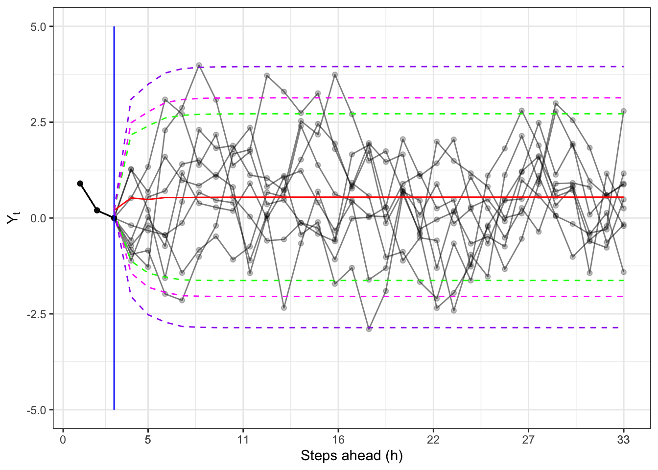
ARMA(1,1) simulation

set.seed(6) # random seed
# *************************************************
#                      Inputs
# *************************************************
# Number of steps ahead
t_bar <- 300
# Intercept
mu <- 0.5
# AR parameters
phi <- c(phi1 = 0.95)
# MA parameters
theta <- c(theta1 = 0.45)
# Variance of the residuals
sigma2_u <- 1
# *************************************************
#                   Simulations
# *************************************************
# Initial value
Yt <- c(mu / (1 - phi[1]))
# Simulated residuals
u_t <- rnorm(t_bar, 0, sqrt(sigma2_u))
# Simulated ARMA(1,1)
for(t in 2:t_bar){
  # AR component
  sum_AR <- phi[1] * Yt[t-1]
  # MA component
  sum_MA <- theta[1] * u_t[t-1]
  # Update Yt
  Yt[t] <- mu + sum_AR + sum_MA + u_t[t]
}

20.1.1 Matrix form

An autoregressive process of order p, AR(p) (Equation 19.3), can be written in matrix form as \[ \mathbf{Y}_t = \mathbf{c} + \mathbf{\Phi} \mathbf{Y}_{t-1} + \mathbf{b} \, u_t \text{,} \] where \[ \underset{\mathbf{Y}_t}{ \underbrace{ \begin{pmatrix} Y_t \\ Y_{t-1} \\ \vdots \\ Y_{t-p+1} \end{pmatrix} }} = \underset{\mathbf{c}}{ \underbrace{ \begin{pmatrix} \mu \\ 0 \\ \vdots \\ 0 \end{pmatrix} }} + \underset{\boldsymbol{\Phi}}{ \underbrace{ \begin{pmatrix} \phi_1 & \phi_2 & \dots & \phi_{p-1} & \phi_p \\ 1 & 0 & \dots & 0 & 0 \\ 0 & 1 & \dots & 0 & 0 \\ \vdots & \vdots & \vdots & \vdots & \vdots \\ 0 & 0 & \dots & 1 & 0 \end{pmatrix} }} \underset{\mathbf{Y}_{t-1}}{ \underbrace{ \begin{pmatrix} Y_{t-1} \\ Y_{t-2} \\ \vdots \\ Y_{t-p} \end{pmatrix} }} + \underset{\mathbf{b}}{ \underbrace{ \begin{pmatrix} 1 \\ 0 \\ \vdots \\ 0 \end{pmatrix} }} \cdot u_t \] where \(\mathbf{Y}_t\), \(\mathbf{c}\) and \(\mathbf{b}\) have dimension \(p \times 1\), while \(\boldsymbol{\Phi}\) is \(p \times p\). The state vector contains \(p\) entries, from \(Y_t\) to \(Y_{t-p+1}\); the lagged state therefore contains \(Y_{t-1}\) to \(Y_{t-p}\).

How to construct the companion matrix \(\boldsymbol{\Phi}\)?

Let’s consider the vector containing the coefficients of the model, i.e. \[ \underset{p \times 1}{\boldsymbol{\gamma}} = \begin{pmatrix} \phi_1 & \phi_2 & \dots & \phi_{p-1} & \phi_p \end{pmatrix} \text{.} \] If the order of the autoregressive process is greater than 1, i.e. \(p > 1\), let’s consider an identity matrix (Equation 31.3) with dimension \((p-1) \times (p-1)\), i.e. \[ \mathbf{I}_{p-1} = \begin{pmatrix} 1 & 0 & \dots & 0 & 0 \\ 0 & 1 & \dots & 0 & 0 \\ \vdots & \vdots & \vdots & \vdots & \vdots \\ 0 & 0 & \dots & 1 & 0 \\ 0 & 0 & \dots & 0 & 1 \end{pmatrix} \text{,} \] and combine it with a column of zeros, i.e. \[ \underset{(p-1) \times p}{\mathbf{L}} = \begin{pmatrix} \mathbf{I}_{p-1} & \mathbf{0}_{(p-1)\times 1} \end{pmatrix} \text{.} \] Finally, add the AR parameters on top of \(\mathbf{L}\), i.e. \[ \underset{p \times p}{\mathbf{\Phi}} = \begin{pmatrix} \boldsymbol{\gamma} \\ \mathbf{L} \end{pmatrix} \text{.} \]

Example: AR(4) in matrix form

Example 20.1 Let’s consider an AR(4) process of the form \[ Y_t = \mu + \phi_1 Y_{t-1} + \phi_2 Y_{t-2} + \phi_3 Y_{t-3} + \phi_4 Y_{t-4} + u_t \text{.} \] Then, the vector containing the coefficients of the model reads \[ \underset{4 \times 1}{\boldsymbol{\gamma}} = \begin{pmatrix} \phi_1 & \phi_2 & \phi_{3} & \phi_4 \end{pmatrix} \text{.} \]

For an AR(4) we start with a diagonal matrix with dimension \(3 \times 3\), i.e. \[ \mathbf{I}_3 = \begin{pmatrix} 1 & 0 & 0 \\ 0 & 1 & 0 \\ 0 & 0 & 1 \end{pmatrix} \text{,} \] and we add a column of zeros, i.e. \[ \underset{3 \times 4}{\mathbf{L}_3} = \begin{pmatrix} 1 & 0 & 0 & 0\\ 0 & 1 & 0 & 0 \\ 0 & 0 & 1 & 0 \end{pmatrix} \text{.} \] and the parameters \[ \underset{4 \times 4}{\mathbf{\Phi}} = \begin{pmatrix} \phi_1 & \phi_2 & \phi_{3} & \phi_4 \\ 1 & 0 & 0 & 0\\ 0 & 1 & 0 & 0 \\ 0 & 0 & 1 & 0 \end{pmatrix} \text{.} \] In order to verify the above result, let’s consider the iteration from \(t-1\) to time \(t\); in matrix form, one obtains \[ \begin{pmatrix} Y_t \\ Y_{t-1} \\ Y_{t-2} \\ Y_{t-3} \end{pmatrix} = \begin{pmatrix} \mu \\ 0 \\ 0 \\ 0 \end{pmatrix} + \begin{pmatrix} \phi_1 & \phi_2 & \phi_{3} & \phi_4 \\ 1 & 0 & 0 & 0\\ 0 & 1 & 0 & 0 \\ 0 & 0 & 1 & 0 \end{pmatrix} \begin{pmatrix} Y_{t-1} \\ Y_{t-2} \\ Y_{t-3} \\ Y_{t-4} \end{pmatrix} + \begin{pmatrix} 1 \\ 0 \\ 0 \\ 0 \end{pmatrix} u_t \text{.} \] After an explicit computation, one can verify that it leads to the classic AR(4) recursion, i.e. \[ \begin{aligned} \begin{pmatrix} Y_t \\ Y_{t-1} \\ Y_{t-2} \\ Y_{t-3} \\ \end{pmatrix} {} & = \begin{pmatrix} \mu \\ 0 \\ 0 \\ 0 \end{pmatrix} + \begin{pmatrix} \phi_1 Y_{t-1} + \phi_2 Y_{t-2} + \phi_3 Y_{t-3} + \phi_4 Y_{t-4} \\ Y_{t-1} \\ Y_{t-2} \\ Y_{t-3} \\ \end{pmatrix} + \begin{pmatrix} u_t \\ 0 \\ 0 \\ 0 \\ \end{pmatrix} \end{aligned} \]

Let’s now consider the matrix form of an ARMA(p,q) process (Equation 20.1), i.e. \[ \mathbf{X}_t = \mathbf{c} + \mathbf{A} \mathbf{X}_{t-1} + \mathbf{b} u_t \text{,} \] where the first component, namely \(Y_t = \mathbf{e}_{p+q}^{\top} \mathbf{X}_t\), is extracted as: \[ Y_t = \mathbf{e}_{1,p+q}^{\top} \mathbf{c} + \mathbf{e}_{1,p+q}^{\top} \mathbf{A} \mathbf{X}_{t-1} + \mathbf{e}_{1,p+q}^{\top} \mathbf{b} \, u_t \text{.} \] where \(\mathbf{e}_{1,p+q}^{\top}\) is the first basis vector (Equation 31.1) with dimension \(p+q\).

\[ \underset{\mathbf{X}_t}{ \underbrace{ \begin{pmatrix} Y_t \\ Y_{t-1} \\ \vdots \\ Y_{t-p+1} \\ u_{t} \\ u_{t-1} \\ \vdots \\ u_{t-q+1} \end{pmatrix} }} = \underset{\mathbf{c}}{ \underbrace{ \begin{pmatrix} \mu \\ 0 \\ 0 \\ \vdots \\ 0 \\ 0 \end{pmatrix} }} + \underset{\mathbf{A}}{ \underbrace{ \begin{pmatrix} \phi_1 & \phi_2 & \dots & \phi_{p-1} & \phi_p & \theta_1 & \theta_2 & \dots & \theta_{q-1} & \theta_q \\ 1 & 0 & \dots & 0 & 0 & 0 & 0 & \dots & 0 & 0 \\ 0 & 1 & \dots & 0 & 0 & 0 & 0 & \dots & 0 & 0 \\ \vdots & \vdots & \vdots & \vdots & \vdots & \vdots & \vdots & \vdots & \vdots & \vdots \\ 0 & 0 & \dots & 1 & 0 & 0 & 0 & \dots & 0 & 0 \\ 0 & 0 & \dots & 0 & 0 & 0 & 0 & \dots & 1 & 0 \end{pmatrix} }} \underset{\mathbf{X}_{t-1}}{ \underbrace{ \begin{pmatrix} Y_{t-1} \\ Y_{t-2} \\ \vdots \\ Y_{t-p} \\ u_{t-1} \\ u_{t-2} \\ \vdots \\ u_{t-q} \end{pmatrix} }} + \underset{\mathbf{b}}{ \underbrace{ \begin{pmatrix} 1 \\ 0 \\ \vdots \\ 0 \\ 1 \\ 0 \\ \vdots \\ 0 \end{pmatrix} }} \cdot u_t \]

How to construct the companion matrix for an ARMA?

Let’s consider the vector \(\gamma\) containing the coefficients of the model, i.e. \[ \underset{1 \times (q+p)}{\boldsymbol{\gamma}} = \begin{pmatrix} \phi_1 & \phi_2 & \dots & \phi_{p-1} & \phi_p & \theta_1 & \theta_2 & \dots & \theta_{q-1} & \theta_q \end{pmatrix} \text{.} \] For an ARMA(p,q), we consider two distinct matrices. For the AR part, we consider the identity matrix (Equation 31.3) with order \(p-1\), i.e. \[ \underset{(p-1) \times (p-1)}{\mathbf{I}_{p-1}} = \begin{pmatrix} 1 & 0 & \dots & 0 & 0 \\ 0 & 1 & \dots & 0 & 0 \\ \vdots & \vdots & \vdots & \vdots & \vdots \\ 0 & 0 & \dots & 1 & 0 \\ 0 & 0 & \dots & 0 & 1 \end{pmatrix} \text{,} \] and we combine it with a column of zeros, i.e. \[ \underset{(p-1) \times p}{\mathbf{L}^{\tiny \text{AR}}} = \begin{pmatrix} \mathbf{I}_{p-1} & \mathbf{0}_{(p-1) \times 1} \end{pmatrix} = \begin{pmatrix} 1 & 0 & \dots & 0 & 0 & 0 \\ 0 & 1 & \dots & 0 & 0 & 0 \\ \vdots & \vdots & \vdots & \vdots & \vdots & 0 \\ 0 & 0 & \dots & 1 & 0 & 0 \\ 0 & 0 & \dots & 0 & 1 & 0 \end{pmatrix} \text{.} \] For the MA part we consider the identity matrix with order \(q-1\), i.e. \[ \mathbf{I}_{q-1} = \begin{pmatrix} 1 & 0 & \dots & 0 & 0 \\ 0 & 1 & \dots & 0 & 0 \\ \vdots & \vdots & \vdots & \vdots & \vdots \\ 0 & 0 & \dots & 1 & 0 \\ 0 & 0 & \dots & 0 & 1 \end{pmatrix} \text{,} \] and we combine it with a column of zeros, i.e. \[ \underset{(q-1) \times q}{\mathbf{L}^{\tiny \text{MA}}} = \begin{pmatrix} \mathbf{I}_{q-1} & \mathbf{0}_{(q-1) \times 1} \end{pmatrix} = \begin{pmatrix} 1 & 0 & \dots & 0 & 0 & 0 \\ 0 & 1 & \dots & 0 & 0 & 0 \\ \vdots & \vdots & \vdots & \vdots & \vdots & 0 \\ 0 & 0 & \dots & 1 & 0 & 0 \\ 0 & 0 & \dots & 0 & 1 & 0 \end{pmatrix} \text{.} \] To combine the matrices \(\mathbf{L}_{p-1}\) and \(\mathbf{L}_{q-1}\), we need to add a matrix of zeros. More precisely: \[ \underset{(q+p-1) \times (q+p)}{\mathbf{L}} = \begin{pmatrix} \mathbf{L}^{\tiny \text{AR}} & \mathbf{0}_{(p-1) \times q } \\ \mathbf{0}_{1 \times p} & \mathbf{0}_{1 \times q} \\ \mathbf{0}_{(q-1) \times p} & \mathbf{L}^{\tiny \text{MA}} \end{pmatrix} \text{.} \] Finally, we combine \(\mathbf{L}\) with the parameters, i.e. \[ \underset{(q+p) \times (q+p)}{\mathbf{A}} = \begin{pmatrix} \boldsymbol{\gamma} \\ \mathbf{L} \end{pmatrix} \text{.} \] Then, the vector \(\mathbf{b}\) is constructed by combining two first basis vectors (Equation 31.1), to ensure it is equal to one in position 1 and in position \(p+1\), i.e. \[ \mathbf{b} = \begin{pmatrix} \mathbf{e}_{1,p} \\ \mathbf{e}_{1,q} \end{pmatrix} \text{.} \]

Example: matrix form of an ARMA(2,3)

Example 20.2 For example, let’s consider an ARMA(2,3): \[ \boldsymbol{\gamma} = \begin{pmatrix} \phi_1 & \phi_2 & \theta_1 & \theta_2 & \theta_3 \end{pmatrix} \text{.} \] The matrix for the AR part is equal to \(\mathbf{\Phi}\) combined with a matrix of zeros, i.e. \[ \underset{1 \times 2}{\mathbf{L}^{\tiny \text{AR}}} = \begin{pmatrix} 1 & 0 \end{pmatrix} \text{,} \] For the MA part, we consider a similar matrix as in the single case but with the first row equal to zero, i.e. \[ \underset{2 \times 3}{\mathbf{L}^{\tiny \text{MA}}} = \begin{pmatrix} 1 & 0 & 0 \\ 0 & 1 & 0 \\ \end{pmatrix} \text{,} \] and we combine \[ \underset{4 \times 5}{\mathbf{L}} = \begin{pmatrix} \mathbf{L}^{\tiny \text{AR}} & \mathbf{0}_{2 \times 3} \\ \mathbf{0}_{1 \times 2} & \mathbf{0}_{1 \times 3} \\ \mathbf{0}_{2 \times 2} & \mathbf{L}^{\tiny \text{MA}} \end{pmatrix} = \begin{pmatrix} 1 & 0 & 0 & 0 & 0 \\ 0 & 0 & 0 & 0 & 0 \\ 0 & 0 & 1 & 0 & 0 \\ 0 & 0 & 0 & 1 & 0 \\ \end{pmatrix} \text{.} \] Finally, we combine \[ \underset{5 \times 5}{\mathbf{A}} = \begin{pmatrix} \boldsymbol{\gamma}\\ \mathbf{L} \end{pmatrix} = \begin{pmatrix} \phi_1 & \phi_2 & \theta_1 & \theta_2 & \theta_3 \\ 1 & 0 & 0 & 0 & 0 \\ 0 & 0 & 0 & 0 & 0 \\ 0 & 0 & 1 & 0 & 0 \\ 0 & 0 & 0 & 1 & 0 \\ \end{pmatrix} \text{.} \] Then, the vector \(\mathbf{b}\) is constructed by combining two vectors \[ \mathbf{b} = \begin{pmatrix} \mathbf{e}_{1,2} \\ \mathbf{e}_{1,3} \end{pmatrix} = \begin{pmatrix} 1 & 0 & 1 & 0 & 0 \end{pmatrix}^{\top} \text{.} \] Let’s check that it leads to a classic ARMA(2,3): \[ \begin{aligned} \begin{pmatrix} Y_t \\ Y_{t-1} \\ u_t \\ u_{t-1} \\ u_{t-2} \\ \end{pmatrix} & {} = \begin{pmatrix} \phi_1 Y_{t-1} + \phi_2 Y_{t-2} + \theta_1 u_{t-1} + \theta_2 u_{t-2} + \theta_3 u_{t-3} \\ Y_{t-1} \\ 0 \\ u_{t-1} \\ u_{t-2} \\ \end{pmatrix} + \begin{pmatrix} u_t \\ 0 \\ u_t \\ 0 \\ 0 \\ \end{pmatrix} \\ & = \begin{pmatrix} \phi_1 Y_{t-1} + \phi_2 Y_{t-2} + \theta_1 u_{t-1} + \theta_2 u_{t-2} + \theta_3 u_{t-3} + u_t \\ Y_{t-1} \\ u_t \\ u_{t-1} \\ u_{t-2} \\ \end{pmatrix} \end{aligned} \]

20.2 Moments

Proposition 20.1 Given the information at time \(t\), the forecasted value at time \(t+h\) for an ARMA(p,q) process reads: \[ \mathbf{X}_{t+h} = \sum_{j = 0}^{h-1} \mathbf{A}^j \mathbf{c} + \mathbf{A}^h \mathbf{X}_{t} + \sum_{j = 0}^{h-1} \mathbf{A}^j \mathbf{b} \, u_{t+h-j} \text{.} \tag{20.2}\]

Proof of Proposition 20.1

Proof. Let’s start developing the Equation 20.2 with \(h = 1\), i.e. \[ \mathbf{X}_{t+1} = \mathbf{c} + \mathbf{A} \mathbf{X}_{t} + \mathbf{b} \, u_{t+1} \text{,} \] with \(h = 2\): \[ \begin{aligned} \mathbf{X}_{t+2} & {} = \mathbf{c} + \mathbf{A} \mathbf{X}_{t+1} + \mathbf{b} \, u_{t+2} = \\ & = \mathbf{c} + \mathbf{A} \left(\mathbf{c} + \mathbf{A} \mathbf{X}_{t} + \mathbf{b} \, u_{t+1} \right) + \mathbf{b} \cdot u_{t+2} = \\ & = \mathbf{c} + \mathbf{A} \mathbf{c} + \mathbf{A}^2 \mathbf{X}_{t} + \mathbf{b} \, u_{t+2} + \mathbf{A} \mathbf{b} \, u_{t+1} \end{aligned} \] with \(h = 3\): \[ \begin{aligned} \mathbf{X}_{t+3} & {} = \mathbf{c} + \mathbf{A} \mathbf{X}_{t+2} + \mathbf{b} \, u_{t+3} = \\ & = \mathbf{c} + \mathbf{A} \left(\mathbf{c} + \mathbf{A} \mathbf{c} + \mathbf{A}^2 \mathbf{X}_{t} + \mathbf{b} \, u_{t+2} + \mathbf{A} \mathbf{b} \, u_{t+1} \right) + \mathbf{b} \, u_{t+3} = \\ & = \mathbf{c} + \mathbf{A} \mathbf{c} + \mathbf{A}^2 \mathbf{c} + \mathbf{A}^3 \mathbf{X}_{t} + \mathbf{b} \, u_{t+3} + \mathbf{A} \mathbf{b} \, u_{t+2} + \mathbf{A}^2 \mathbf{b} \, u_{t+1} \end{aligned} \] and so on. Hence, when the companion matrix is stable, the impact of shocks decreases over time.

Proposition 20.2 (Expectation of an ARMA) The conditional expectation at time \(t+h\) of \(\mathbf{X}_{t+h}\) given the information up to time \(t\) can be easily computed from Equation 20.2, i.e. \[ \mathbb{E}\{\mathbf{X}_{t+h}\mid \mathcal{F}_t \} = (\mathbf{I}_{p+q} - \mathbf{A}^h) \ (\mathbf{I}_{p+q} - \mathbf{A})^{-1}\mathbf{c} + \mathbf{A}^h \mathbf{X}_{t} \text{.} \]

Proof of Proposition 20.2

Proof. The expectation of Equation 20.2 reads: \[ \mathbb{E}\{\mathbf{X}_{t+h}\mid \mathcal{F}_t \} = \sum_{j = 0}^{h-1} \mathbf{A}^j \mathbf{c} + \mathbf{A}^h \mathbf{X}_{t} + \sum_{j = 0}^{h-1} \mathbf{A}^j \mathbf{b} \cdot \mathbb{E}\{u_{t+h-j} \mid \mathcal{F}_t \} \text{.} \] Under the assumption that \(u_{t+h-j} \sim \text{MDS}(0,1)\), we have that for all \(t\) \[ \mathbb{E}\{u_{t+1} \mid \mathcal{F}_{t} \} = 0 \text{.} \] Therefore \[ \mathbb{E}\{\mathbf{X}_{t+h}\mid \mathcal{F}_t \} = \sum_{j = 0}^{h-1} \mathbf{A}^j \mathbf{c} + \mathbf{A}^h \mathbf{X}_{t} \text{,} \] where for constant \(\mathbf{c}\), the series further simplifies in \[ \sum_{j = 0}^{h-1} \mathbf{A}^j \mathbf{c} = (\mathbf{I}_{p+q} - \mathbf{A}^h) \ (\mathbf{I}_{p+q} - \mathbf{A})^{-1} \mathbf{c} \text{,} \] with \(\mathbf{I}_{p+q}\) the identity matrix (Equation 31.3).

Proposition 20.3 (Variance of an ARMA) Taking the variance of Equation 20.2 on both sides gives \[ \mathbb{V}\{\mathbf{X}_{t+h}\mid \mathcal{F}_t \} = \sigma_{\text{u}}^2 \sum_{j = 0}^{h-1} \mathbf{A}^j \mathbf{b} \mathbf{b}^{\top} (\mathbf{A}^j)^{\top} \text{.} \] Moreover, assuming \(u_t \sim \text{WN}(0, \sigma_{\text{u}}^2)\) and independence across time, the conditional covariance is: \[ \mathbb{C}v\{\mathbf{X}_{t+h}, \mathbf{X}_{t+k} \mid \mathcal{F}_t \} = \sigma_{\text{u}}^2 \sum_{j=0}^{\min(h,k)-1} \mathbf{A}^{h-1-j} \mathbf{b} \mathbf{b}^{\top} (\mathbf{A}^{k-1-j})^{\top}. \]

Proof of Proposition 20.3

Proof. Taking the conditional variance gives \[ \mathbb{V}\{\mathbf{X}_{t+h}\mid \mathcal{F}_t \} = \sum_{j = 0}^{h-1} \mathbb{V}\{\mathbf{A}^j \mathbf{b} \, u_{t+h-j} \mid \mathcal{F}_t \} = \sum_{j = 0}^{h-1} \mathbf{A}^j \mathbf{b} \mathbb{V}\{u_{t+h-j} \mid \mathcal{F}_t \} \mathbf{b}^{\top} (\mathbf{A}^j)^{\top} \text{.} \] Then, if \(u_t\) is a White Noise process, its variance is constant, hence independent from \(t\), and equal to \(\sigma_{\text{u}}^2\). For the covariance formula, each \(\mathbf{X}_{t+h}\) is influenced by past shocks \(u_{t+h-j}\). Since the shocks are uncorrelated across time, only shared shocks affect both \(\mathbf{X}_{t+h}\) and \(\mathbf{X}_{t+k}\). The number of common shocks is \(\min(h, k)\), and each contributes: \[ \mathbb{C}v\{\mathbf{A}^{h-1-j} \mathbf{b} u_{t+1+j}, \mathbf{A}^{k-1-j} \mathbf{b} u_{t+1+j} \} = \sigma_{\text{u}}^2 \mathbf{A}^{h-1-j} \mathbf{b} \mathbf{b}^\top (\mathbf{A}^{k-1-j})^\top \text{.} \]

Example: ARMA(2,3) iterative forecast

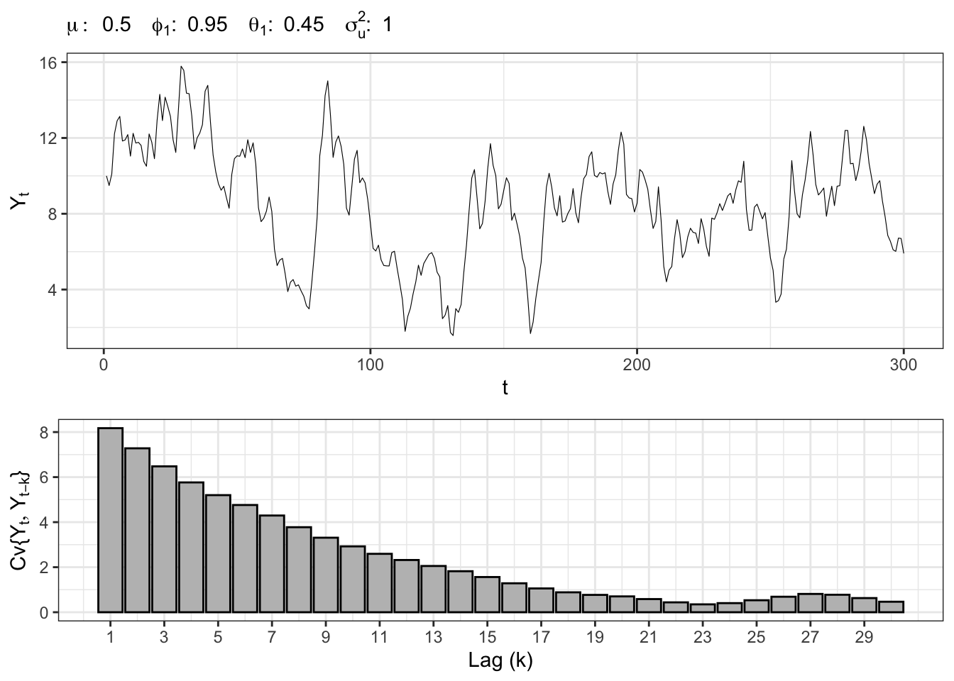
Example 20.3 Let’s use Monte Carlo simulations to establish if the results are accurate.

simulate_ARMA

# Simulate an ARMA(p, q) process
simulate_ARMA <- function(t_bar, nsim = 1, mu = 0, phi = c(0.5, 0.2), theta = c(0.4, 0.1), sigma2 = 1, y0, eps0){
  scenarios <- list()
  # MA order
  q <- length(theta)
  # AR order
  p <- length(phi)
  # Initial lag to start
  i_start <- max(c(p, q)) + 1
  for(sim in 1:nsim){
    # Simulated residuals
    if (!missing(eps0)){
      eps <- c(eps0, rnorm(t_bar - q, sd = sqrt(sigma2)))
    } else {
      eps <- rnorm(t_bar, sd = sqrt(sigma2))
    }
    # Initialize the simulation
    if (!missing(y0)){
      x <- c(y0)
    } else {
      x <- eps
    }
    for(t in i_start:t_bar){
      # AR part
      ar_part <- 0
      for(i in 1:length(phi)){
        ar_part <- ar_part + phi[i] * x[t-i]
      }
      # MA part
      ma_part <- 0
      for(i in 1:length(theta)){
        ma_part <- ma_part + theta[i] * eps[t-i]
      }
      # Next step simulation
      x[t] <- mu + ar_part + ma_part + eps[t]
    }
    scenarios[[sim]] <- x
  }
  scenarios
}

pow_matrix

# Compute the power of a matrix
pow_matrix <- function(x, n = 0){
  M <- x
  # Case power == 0
  if (n == 0) {
    M <- diag(1, nrow(M), ncol(M))
  } else if(n > 1) {
    M_pow <- M
    for(i in 2:n){
      M_pow <- M_pow %*% M
    }
    M <- M_pow
  }
  return(M)
}

expectation_ARMA

# Compute the expected value with the iterative formula
expectation_ARMA <- function(X0, h = 10, A, b, c){
  A_h <- pow_matrix(A, h)
  I_p <- diag(1, nrow = nrow(A_h))
  (I_p - A_h) %*% solve(I_p - A) %*% c  + A_h %*% X0
}

covariance_ARMA

# Compute the covariance with the iterative formula
covariance_ARMA <- function(h, k, A, b, sigma2 = 1){
  cv_x <- 0
  for(j in 0:(min(h, k)-1)){
    A_hj <- pow_matrix(A, h-1-j)
    A_kj <- pow_matrix(A, k-1-j)
    cv_x <- cv_x + A_hj %*% b %*% t(b) %*% t(A_kj)
  }
  sigma2 * cv_x
}

ARMA moments

# *************************************************
#                      Inputs
# *************************************************
set.seed(6) # random seed
nsim <- 200 # Number of simulations
t_bar <- 100000 # Steps for each simulation
phi <- c(0.3, 0.15) # AR parameters
theta <- c(0.3, 0.15, 0.1) # MA parameters
mu <- 0.3 # Intercept
sigma2 <- 1 # Variance of the residuals
y0 <- c(0.9, 0.2, 0) # Initial values for y0
eps0 <- c(0.3, -0.2, 0.1) # Initial values for eps0
h <- 200 # Number of steps ahead
# *************************************************
#                   Simulations
# *************************************************
scenarios <- simulate_ARMA(t_bar, nsim, mu, phi, theta,
                           sigma2, y0, eps0)
# Build companion matrix
L_AR <- matrix(c(1, 0, 0, 0, 0), nrow = 1)
L_MA <- cbind(c(0, 0), c(0, 0), diag(2), c(0, 0))
A <- rbind(c(phi, theta), L_AR, rep(0, 5), L_MA)
# Build vector b
b <- matrix(c(1, 0, 1, 0, 0), ncol = 1)
# Build vector c
c <- matrix(c(mu, 0, 0, 0, 0), ncol = 1)
# *************************************************
#                      Moments
# *************************************************
# Compute expectation and variances with Monte Carlo
e_mc <- mean(purrr::map_dbl(scenarios, ~mean(.x)))
v_mc <- mean(purrr::map_dbl(scenarios, ~var(.x)))
cv_mc_L1 <- mean(purrr::map_dbl(scenarios, ~cov(.x[-1], lag(.x, 1)[-1])))
cv_mc_L2 <- mean(purrr::map_dbl(scenarios, ~cov(.x[-c(1,2)], lag(.x, 2)[-c(1,2)])))
cv_mc_L3 <- mean(purrr::map_dbl(scenarios, ~cov(.x[-c(1:3)], lag(.x, 3)[-c(1:3)])))
cv_mc_L4 <- mean(purrr::map_dbl(scenarios, ~cov(.x[-c(1:4)], lag(.x, 4)[-c(1:4)])))
cv_mc_L5 <- mean(purrr::map_dbl(scenarios, ~cov(.x[-c(1:5)], lag(.x, 5)[-c(1:5)])))
# Compute expectation and variances with Formula
# State vector for forecasting
X0 = c(y0[-3][c(2,1)], eps0[c(3:1)])
e_mod <- expectation_ARMA(X0, h = h, A, b, c)[1,1]
v_mod <- covariance_ARMA(h, h, A, b, sigma2)[1,1]
cv_mod_L1 <- covariance_ARMA(h, h-1, A, b, sigma2 = 1)[1,1]
cv_mod_L2 <- covariance_ARMA(h, h-2, A, b, sigma2 = 1)[1,1]
cv_mod_L3 <- covariance_ARMA(h, h-3, A, b, sigma2 = 1)[1,1]
cv_mod_L4 <- covariance_ARMA(h, h-4, A, b, sigma2 = 1)[1,1]
cv_mod_L5 <- covariance_ARMA(h, h-5, A, b, sigma2 = 1)[1,1]

Covariance	Formula	Monte Carlo
\(\mathbb{E}\{Y_t\}\)	0.5454545	0.5451268
\(\mathbb{V}\{Y_t\}\)	1.7466575	1.7472189
\(\mathbb{C}v\{Y_t, Y_{t-1}\}\)	1.1317615	1.1322251
\(\mathbb{C}v\{Y_t, Y_{t-2}\}\)	0.8115271	0.8118819
\(\mathbb{C}v\{Y_t, Y_{t-3}\}\)	0.5132223	0.5133504
\(\mathbb{C}v\{Y_t, Y_{t-4}\}\)	0.2756958	0.2758340
\(\mathbb{C}v\{Y_t, Y_{t-5}\}\)	0.1596921	0.1596755

Table 20.1: Theoretical long-term moments and moments computed on 200 Monte Carlo simulations (t = 100000).

Figure 20.2: ARMA(2,3) simulations with expected value (red) and confidence intervals with \(\alpha = 0.1\) (green), \(\alpha = 0.05\) (blue) and \(\alpha = 0.01\) (deep blue).