library(dplyr)# required for figureslibrary(ggplot2)library(gridExtra)# required to render latexlibrary(backports)library(latex2exp)# required for render tableslibrary(knitr)library(kableExtra)# Random seedset.seed(1)
19.1 MA(q)
In time series analysis, a univariate time series \(Y_t\) is defined as a Moving Average process with order q (MA(q)) when it satisfies the difference equation, i.e. \[
Y_t = u_{t} + \theta_1 u_{t-1} + \dots + \theta_q u_{t-q}
\text{,}
\tag{19.1}\] where \(u_t \sim \text{WN}(0, \sigma_{\text{u}}^2)\) (Definition 18.5). An MA(q) process can be equivalently expressed as a polynomial in \(\theta\) of the Lag operator (Equation 18.7), i.e. \[
Y_t = \Theta(L) u_t, \quad u_t \sim \text{WN}(0, \sigma_{\text{u}}^2)
\text{,}
\] where \(\Theta(L)\) is a polynomial of the form \(\Theta(L) = 1 + \theta_1 L + \dots + \theta_q L^q\). Given this representation, it is clear that an MA(q) process is stationary independently of the value of the parameters. Moreover, the stationary process \(Y_t\) admits an infinite moving average or MA(\(\infty\)) representation (see Wold (1939)) if it satisfies the difference equation, i.e. \[
Y_t = \Psi(L) u_{t} = u_{t} + \psi_1 u_{t-1} + \dots = \sum_{j = 0}^{\infty} \psi_j u_{t-j}, \qquad \psi_0 = 1
\text{,}
\] under the following summability condition the process is covariance stationary; with standard regularity conditions on the innovations, it is also ergodic, i.e. \[
\sum_{j = 0}^{\infty} |\psi_j| < \infty
\text{.}
\] If the above condition holds, then the MA(\(\infty\)) process can be written in compact form as: \[
Y_t = \Psi(L) u_t, \quad u_t \sim \text{WN}(0, \sigma_{\text{u}}^2), \; \Psi(L) = \sum_{j = 0}^{\infty} \psi_j L^j
\text{.}
\]
Proposition 19.1 (Expectation of an MA(q)) In general, the expected value of an MA(q) process depends on the distribution of \(u_t\). Under the standard assumption that \(u_t\) is a White Noise (Equation 18.1), its expected value is equal to zero for every \(t\), i.e. \[
\mathbb{E}\{Y_t\} = \sum_{i = 0}^{q} \theta_i \mathbb{E}\{u_{t-i}\} = 0
\text{.}
\]
Proof. Given a process \(Y_t\) such that \(\mathbb{E}\{Y_t\} = \mu\), it is always possible to simply reparametrize the Equation 19.1 as: \[
Y_t = \mu + u_{t} + \theta_1 u_{t-1} + \dots + \theta_q u_{t-q}
\text{,}
\] or rescale the process, i.e. \(\tilde{Y}_t = Y_t - \mu\), and work with a process with zero mean. Then, let’s consider an MA process of order q; the expectation of the process is computed as \[
\begin{aligned}
\mathbb{E}\{Y_t\} & {} = \mathbb{E}\left\{u_{t} + \sum_{i = 1}^{q} \theta_i u_{t-i}\right\} = \sum_{i = 0}^{q} \theta_i \mathbb{E}\{u_{t-i}\} = 0
\end{aligned}
\text{.}
\] Hence, the expected value of \(Y_t\) depends on the expected value of the residuals \(u_t\), which under the White Noise assumption is zero for every \(t\).
Proposition 19.2 (Autocovariance of an MA(q)) For every lag \(k > 0\), the autocovariance function, denoted as \(\gamma_k\), is defined as: \[
\begin{aligned}
\gamma_k & {} = \mathbb{C}v\{Y_t, Y_{t-k}\} =
\begin{cases}
\sigma_{\text{u}}^2 \sum_{j = 0}^{q-k} \theta_j \theta_{j+k} & k \le q \\
0 & k > q
\end{cases}
\end{aligned}
\text{.}
\] where by convention \(\theta_0 = 1\).
The covariance is different from zero only when the lag \(k\) is less than or equal to the order of the process \(q\). Setting \(k = 0\), one obtains the variance \(\mathbb{V}\{Y_t\}\), i.e. \[
\gamma_0 = \sigma_{\text{u}}^2 \sum_{i = 0}^{q} \theta_i^2 = \sigma_{\text{u}}^2 (1 + \theta_1^2 + \dots + \theta_q^2)
\text{.}
\] It follows that the autocorrelation function is bounded up to the lag \(q\), i.e. \[
\rho_k =
\begin{cases}
1 & k = 0 \\
\frac{\sigma_{\text{u}}^2 \sum_{j = 0}^{q-k} \theta_j \theta_{j+k}}{\sigma_{\text{u}}^2 (1 + \theta_1^2 + \dots + \theta_q^2)} & 0 < k \le q \\
0 & k > q
\end{cases}
\] where \(\rho_k = \mathbb{C}r\{Y_t, Y_{t-k}\}\).
19.1.1 MA(1)
Proposition 19.3 (Moments of an MA(1)) Let’s consider a process \(Y_t \sim \text{MA}(1)\), i.e. \[
Y_t = \mu + \theta_1 u_{t-1} + u_{t}
\text{.}
\] Independently from the specific distribution of \(u_t\), the process has to be a White Noise, hence with expected value equal to zero. Therefore, the expectation of an MA(1) process is equal to \(\mu\), i.e. \(\mathbb{E}\{Y_t\} = \mu\). The variance instead is equal to \[
\gamma_0 = \mathbb{V}\{Y_t\} = \sigma_{\text{u}}^2(1+\theta_{1}^2)
\text{.}
\] In general, the autocovariance function for order \(k\) is defined as \[
\gamma_k = \mathbb{C}v\{Y_t, Y_{t-k}\} =
\begin{cases}
\theta_{1} \sigma_{\text{u}}^2 & k = 1 \\
0 & k > 1
\end{cases}
\] It follows that the autocovariance function is bounded up to the first lag, i.e. \[
\sum_{k = 0}^{\infty} |\gamma_{k}| = \sigma_{\text{u}}^2 (1 + \theta_{1}^2 + |\theta_{1}|)
\text{,}
\] and therefore the process is always stationary without requiring any condition on the parameter \(\theta_1\). Also, the autocorrelation is different from zero only between the first two lags, i.e. the process is said to have a short memory\[
\rho_k = \mathbb{C}r\{Y_t, Y_{t-k}\} =
\begin{cases}
1 & k = 0 \\
\frac{\theta_{1}}{1 + \theta_{1}^2} & k = 1 \\
0 & k > 1
\end{cases}
\]
Proof. Let’s consider an MA(1) process \(Y_t = \mu + \theta_1 u_{t-1} + u_{t}\), where \(u_t\) is a White Noise process (Equation 18.1). The expected value of \(Y_t\) depends on the intercept \(\mu\), i.e. \[
\mathbb{E}\{Y_t\} = \mu + \theta_1 \mathbb{E}\{u_{t-1}\} + \mathbb{E}\{u_{t}\} = \mu
\text{.}
\] Under the White Noise assumption the residuals are uncorrelated, hence the variance is computed as \[
\begin{aligned}
\gamma_0 {} & = \mathbb{V}\{\mu + u_{t} + \theta_1 u_{t-1}\} = \\
& = \mathbb{V}\{u_{t} + \theta_1 u_{t-1}\} = \\
& = \mathbb{V}\{u_{t}\} + \theta_1^2 \mathbb{V}\{u_{t-1}\} = \\
& = \sigma_{\text{u}}^2 + \theta_{1}^2 \sigma_{\text{u}}^2 = \\
& = \sigma_{\text{u}}^2 (1+\theta_{1}^2)
\end{aligned}
\] By definition, the autocovariance function between time \(t\) and a generic lagged value \(t-k\) reads \[
\begin{aligned}
\gamma_k {} & = \mathbb{C}v\{Y_t, Y_{t-k}\} \\
& = \mathbb{E}\{Y_t Y_{t-k}\} - \mathbb{E}\{Y_t\} \mathbb{E}\{Y_{t-k}\} = \\
& = \mathbb{E}\{(\mu + u_{t} + \theta_{1}u_{t-1} )(\mu +u_{t-k} + \theta_{1}u_{t-k-1})\} - \mu^2= \\
& = \mathbb{E}\{u_{t} u_{t-k}\} + \theta_{1}\mathbb{E}\{ u_{t-k} u_{t-1}\} +
\theta_{1} \mathbb{E}\{u_t u_{t-k-1} \} + \theta_1^2 \mathbb{E}\{u_{t-1} u_{t-k-1}\} + \\
& \quad\; + \mu^2 + \mu \mathbb{E}\{u_{t-k}\} + \mu \theta_1 \mathbb{E}\{u_{t-k-1}\} + \mu \mathbb{E}\{u_{t}\} + \mu \theta_1 \mathbb{E}\{u_{t-1}\} = \\
& =
\begin{cases}
\sigma_{\text{u}}^2 (1+\theta_1^2) & k = 0 \\
\theta_{1}\sigma_{\text{u}}^2 & k = 1 \\
0 & k > 1
\end{cases}
\end{aligned}
\] This is a consequence of \(u_t\) being a White Noise and so uncorrelated in time, i.e. \(\mathbb{E}\{u_t u_{t-k}\} = 0\) for every \(k \ne 0\). This implies that the correlation between two lags is also zero if \(k > 1\).
Example: stationary MA(1)
Example 19.1 Under the assumption that the residuals are Gaussian, i.e. \(u_t \sim \mathcal{N}(0, \sigma_{\text{u}}^2)\), we can simulate scenarios of a moving-average process of order 1 of the form \[
Y_t \sim \text{MA}(1) \iff Y_t = \mu + \theta_1 u_{t-1} + u_{t}
\text{.}
\tag{19.2}\]
MA(1) simulation
set.seed(1) # random seed# *************************************************# Inputs# *************************************************# Number of stepst_bar <-100000# Long term meanmu <-1# MA parameterstheta <-c(theta1 =0.15)# Variance residualssigma2_u <-1# *************************************************# Simulation# *************************************************# InitializationYt <-c(mu)# Simulated residualsu_t <-rnorm(t_bar, 0, sqrt(sigma2_u))# Simulated MA(1) processfor(t in2:t_bar){ Yt[t] <- mu + theta[1]*u_t[t-1] + u_t[t]}
Table 19.1: Empirical and theoretical expectation, variance, covariance and correlation (first lag) for a stationary MA(1) process.
19.2 AR(P)
In time series analysis, a univariate time series \(Y_t\) is defined as an autoregressive process of order p (AR(p)) when it satisfies the difference equation, i.e. \[
Y_t = \mu + \phi_1 Y_{t-1} + \dots + \phi_p Y_{t-p} + u_t
\text{,}
\tag{19.3}\] where \(p\) defines the order of the process and \(u_t \sim \text{WN}(0, \sigma_{\text{u}}^2)\). In compact form: \[
Y_t = \mu + \sum_{i=1}^{p}\phi_{i} Y_{t-i} + u_{t}
\text{.}
\] An autoregressive process can be equivalently expressed in terms of the polynomial operator, i.e. \[
\Phi(L) Y_t = \mu + u_t \text{,}\quad \Phi(L) = 1 - \phi_1 L - \dots - \phi_p L^p
\text{.}
\] From Section 18.3.1 it follows that a stationary AR(p) process exists if and only if all the solutions of the characteristic equations, i.e. \(\Phi(z) = 0\), are greater than 1 in absolute value. In such a case, the AR(p) process admits an equivalent representation in terms of MA(\(\infty\)), i.e. \[
\begin{aligned}
Y_t - \mathbb{E}\{Y_t\} & {} = \Phi(L)^{-1} u_t = \frac{1}{1-\phi_1 L - \dots -\phi_p L^p} u_t \\
& = (1 + \psi_1 L + \psi_2 L^2 + \dots)u_t = \sum_{i = 0}^{\infty} \psi_i u_{t-i} \text{.}
\end{aligned}
\]
Proposition 19.4 (Expectation of an AR(p)) The unconditional expected value of a stationary AR(p) process reads \[
\mathbb{E}\{Y_t\} = \frac{\mu}{1-\sum_{i=1}^{p}\phi_{i} }
\text{.}
\]
Proof. Let’s consider an AR(p) process \(Y_t\), then the unconditional expectation of the process is computed as \[
\begin{aligned}
\mathbb{E}\{Y_t\} & {} = \mathbb{E}\left\{\mu + \sum_{i=1}^{p}\phi_{i} Y_{t-i} + u_{t}\right\} = \\
& = \mu + \sum_{i = 1}^{p} \phi_i \mathbb{E}\{Y_{t-i}\} + \mathbb{E}\{u_{t}\} = \\
& = \mu + \sum_{i = 1}^{p} \phi_i \mathbb{E}\{Y_{t}\}
\end{aligned}
\] Since, under the assumption of stationarity, the long-term expectation of \(\mathbb{E}\{Y_{t-i}\}\) is the same as the long-term expectation of \(\mathbb{E}\{Y_{t}\}\). Hence, solving for the expected value, one obtains: \[
\mathbb{E}\{Y_t\} \left(1- \sum_{i = 1}^{p} \phi_i\right) = \mu
\implies \mathbb{E}\{Y_{t}\} = \frac{\mu}{1-\sum_{i=1}^{p}\phi_{i}}
\text{.}
\]
If the AR(p) process is stationary, the covariance function satisfies the recursive relation, i.e. \[
\begin{cases}
\gamma_k - \phi_1 \gamma_{k-1} - \dots - \phi_p\gamma_{k-p} = 0 \\
\; \vdots \\
\gamma_0 = \phi_1 \gamma_1 + \dots + \phi_p \gamma_p + \sigma_{\text{u}}^2
\end{cases}
\] where \(\gamma_{-k} = \gamma_{k}\). For \(k = 0, \dots, p\), the above equations form a system of \(p+1\) linear equations in \(p + 1\) unknowns \(\gamma_{0}, \dots, \gamma_{p}\), also known as Yule-Walker equations.
Proposition 19.5 (Variance of an AR(1)) Let’s consider an AR(1) model without intercept so that \(\mathbb{E}\{Y_t\}=0\). Then, its covariance function reads: \[
\gamma_k = \frac{\sigma_{\text{u}}^2}{1-\phi_1^2} \phi_1^k = \gamma_0 \phi_1^k
\text{.}
\]
Proof. Let’s consider an AR(1) model without intercept so that \(\mathbb{E}\{Y_t\}=0\), i.e. \[
Y_t = \phi_1 Y_{t-1} + u_t
\text{.}
\] The proof of the covariance function is divided in two parts. Firstly, we compute the variance and covariances of the AR(1) model. Then, we set the system and we solve it. Notably, the variance of \(Y_t\) reads: \[
\begin{aligned}
\gamma_0 = \mathbb{V}\{Y_t\} & {} = \mathbb{E}\{Y_t^2\} - \mathbb{E}\{Y_t\}^2 = \mathbb{E}\{Y_t^2\} = \\
& = \mathbb{E}\{Y_t (\phi_1 Y_{t-1} + u_t )\} = \\
& = \phi_1 \mathbb{E}\{Y_t Y_{t-1}\} + \mathbb{E}\{Y_t u_t\} = \\
& = \phi_1 \gamma_1 + \sigma_{\text{u}}^2
\end{aligned}
\tag{19.4}\] remembering that \(\mathbb{E}\{Y_{t} u_t\} = \mathbb{E}\{u_t^2\}\). The covariance with first lag, namely \(\gamma_1\) is computed as: \[
\begin{aligned}
\gamma_1 = \mathbb{C}v\{Y_t, Y_{t-1}\} & {} = \mathbb{E}\{(\phi_1 Y_{t-1} + u_t)Y_{t-1}\} = \\
& = \phi_1 \mathbb{E}\{Y_{t-1}^2\} = \phi_1 \gamma_0
\end{aligned}
\tag{19.5}\] The Yule-Walker system is given by Equation 19.4, Equation 19.5, i.e. \[
\begin{cases}
\gamma_0 = \phi_1 \gamma_1 + \sigma_{\text{u}}^2 & (L_0) \\
\gamma_1 = \phi_1 \gamma_0 & (L_1)
\end{cases}
\] In order to solve the system, let’s substitute \(\gamma_1\) (Equation 19.5) in \(\gamma_0\) (Equation 19.4) and solve for \(\gamma_0\), i.e. \[
\begin{cases}
\gamma_0 = \phi_1^2 \gamma_0 + \sigma_{\text{u}}^2 = \frac{\sigma_{\text{u}}^2}{1-\phi_1^2} & (L_0) \\
\gamma_1 = \phi_1 \frac{\sigma_{\text{u}}^2}{1-\phi_1^2} & (L_1)
\end{cases}
\] Hence, by the relation \(\gamma_k = \phi_1 \gamma_{k-1}\) the covariance reads explicitly: \[
\gamma_k = \frac{\sigma_{\text{u}}^2}{1-\phi_1^2} \phi_1^k = \gamma_0 \phi_1^k
\text{.}
\]
Proposition 19.6 (Variance of an AR(2)) Let’s consider an AR(2) model without intercept so that \(\mathbb{E}\{Y_t\}=0\). Then, its covariance function reads: \[
\gamma_k =
\begin{cases}
\gamma_0 = \psi_0 \sigma_{\text{u}}^2 & k = 0 \\
\gamma_1 = \psi_1 \gamma_0 & k = 1 \\
\gamma_2 = \psi_2 \gamma_0 & k = 2 \\
\gamma_k = \phi_1 \gamma_{k-1} + \phi_2 \gamma_{k-2} & k \ge 3 \\
\end{cases}
\] where \[
\begin{aligned}
& {} \psi_0 = (1-\phi_1 \psi_1 - \phi_2 \psi_2)^{-1} \\
& \psi_1 = \phi_1(1-\phi_2)^{-1} \\
& \psi_2 = \psi_1 \phi_1 + \phi_2
\end{aligned}
\]
# *************************************************# Inputs# *************************************************# Number of simulationsnsim <-500# Horizon for each simulationt_bar <-100000# AR(4) parametersphi <-c(0.3, 0.15, 0.1, 0.03)# Variance of the residualssigma2 <-1# *************************************************# Simulations# *************************************************scenarios <- purrr::map(1:nsim, ~AR4_simulate(t_bar, phi, sigma2))# *************************************************# Moments# *************************************************# Compute variance and covariances with Monte Carlov_mc <-mean(purrr::map_dbl(scenarios, ~var(.x)))cv_mc_L1 <-mean(purrr::map_dbl(scenarios, ~cov(.x[-1], lag(.x, 1)[-1])))cv_mc_L2 <-mean(purrr::map_dbl(scenarios, ~cov(.x[-c(1,2)], lag(.x, 2)[-c(1,2)])))cv_mc_L3 <-mean(purrr::map_dbl(scenarios, ~cov(.x[-c(1:3)], lag(.x, 3)[-c(1:3)])))cv_mc_L4 <-mean(purrr::map_dbl(scenarios, ~cov(.x[-c(1:4)], lag(.x, 4)[-c(1:4)])))cv_mc_L5 <-mean(purrr::map_dbl(scenarios, ~cov(.x[-c(1:5)], lag(.x, 5)[-c(1:5)])))# Compute variance and covariances with formulasv_mod <-AR4_covariance(phi, sigma2, lags =0)[1]cv_mod_L1 <-AR4_covariance(phi, sigma2, lags =1)[2]cv_mod_L2 <-AR4_covariance(phi, sigma2, lags =2)[3]cv_mod_L3 <-AR4_covariance(phi, sigma2, lags =3)[4]cv_mod_L4 <-AR4_covariance(phi, sigma2, lags =4)[5]cv_mod_L5 <-AR4_covariance(phi, sigma2, lags =5)[6]
Covariance
Formula
MonteCarlo
\(\mathbb{V}\{Y_t\}\)
1.2510514
1.2509967
\(\mathbb{C}v\{Y_t, Y_{t-1}\}\)
0.5004128
0.5002624
\(\mathbb{C}v\{Y_t, Y_{t-2}\}\)
0.3998174
0.3996579
\(\mathbb{C}v\{Y_t, Y_{t-3}\}\)
0.3351247
0.3349660
\(\mathbb{C}v\{Y_t, Y_{t-4}\}\)
0.2480828
0.2482111
\(\mathbb{C}v\{Y_t, Y_{t-5}\}\)
0.1796877
0.1797934
Table 19.4: Theoretical long-term variance and covariances computed on 500 Monte Carlo simulations (t = 100000).
19.2.1 Stationary AR(1)
Let’s consider an AR(1) process, i.e. \[
Y_t = \mu + \phi_{1} Y_{t-1} + u_{t}
\text{.}
\] Through recursion up to time 0 it is possible to express an AR(1) model as an \(\text{MA}(\infty)\), i.e. \[
Y_t = \phi_1^{t} Y_0 + \mu \sum_{j=0}^{t-1} \phi_{1}^{j} + \sum_{j = 0}^{t-1} \phi_{1}^{j} u_{t-j}
\text{,}
\] where the process is stationary if and only if \(|\phi_1|<1\). In fact, independently from the specific distribution of the residuals \(u_t\), the unconditional expectation of an AR(1) converges if and only if \(|\phi_1|<1\), i.e. \[
\mathbb{E}\{Y_t \mid Y_0\} = \phi_1^{t} Y_0 + \mu \sum_{j=0}^{t-1} \phi_{1}^{j}
= \phi_1^t Y_0 + \mu\frac{1-\phi_1^t}{1-\phi_1} \xrightarrow[t\to\infty]{} \frac{\mu}{1-\phi_1}
\text{.}
\] The variance instead is computed as: \[
\mathbb{V}\{Y_t \mid Y_0\} = \sigma_{\text{u}}^{2}\sum_{j=0}^{t-1} \phi_{1}^{2j}
= \sigma_{\text{u}}^2\frac{1-\phi_1^{2t}}{1-\phi_1^2} \xrightarrow[t\to\infty]{} \gamma_0 = \frac{\sigma_{\text{u}}^{2}}{1-\phi_{1}^2}
\text{.}
\] The autocovariance decays exponentially fast depending on the parameter \(\phi_1\), i.e. \[
\gamma_1 = \mathbb{C}v\{Y_t, Y_{t-1}\} = \phi_{1} \cdot \frac{\sigma_{\text{u}}^{2}}{1-\phi_{1}^2} = \phi_1 \cdot \gamma_0
\text{,}
\] where in general for the lag \(k\)\[
\gamma_k = \mathbb{C}v\{Y_t, Y_{t-k}\} = \phi_{1}^{|k|} \cdot \gamma_0
\text{.}
\] Finally, the autocorrelation function \[
\rho_{1} = \mathbb{C}r\{Y_t, Y_{t-1}\} = \frac{\gamma_1}{\gamma_0} = \phi_1
\text{,}
\] where in general for the lag \(k\)\[
\rho_{k} = \mathbb{C}r\{Y_t, Y_{t-k}\} = \phi_{1}^{|k|}
\text{.}
\] An example of a simulated AR(1) process (\(\phi_1 = 0.95\), \(\mu = 0.5\) and \(\sigma_{\text{u}}^2 = 1\) and Normally distributed residuals) with its covariance function is shown in Figure 19.2.
Figure 19.2: AR(1) simulation and expected value (red) on the top. Empirical autocovariance (gray) and fitted exponential decay (blue) at the bottom.
AR(1) simulation
set.seed(1) # random seed# *************************************************# Inputs# *************************************************# Number of stepst_bar <-100000# Long term meanmu <-0.5# AR parametersphi <-c(phi1 =0.95)# Variance residualssigma2_u <-1# *************************************************# Simulation# *************************************************# InitializationYt <-c(mu)# Simulated residualsu_t <-rnorm(t_bar, 0, sqrt(sigma2_u))# Simulated AR(1) processfor(t in2:t_bar){ Yt[t] <- mu + phi[1]*Yt[t-1] + u_t[t]}
Example: sampling from a stationary AR(1)
Example 19.2 Sampling the process for different \(t\) we expect that, on a large number of simulations, the distribution will be normal with stationary moments, i.e. for all \(t\)\[
Y_t \sim \mathcal{N}\left(\frac{\mu}{1-\phi_{1}}, \frac{\sigma_{\text{u}}^{2}}{1-\phi_{1}^2} \right) \text{.}
\]
Simulate and sample a stationary AR(1)
# *************************************************# Inputs# *************************************************set.seed(3) # random seedt_bar <-120# number of steps aheadj_bar <-1000# number of simulationssigma <-1# standard deviation of epsilonpar <-c(mu =0, phi1 =0.7) # parametersy0 <- par[1]/(1-par[2]) # initial pointt_sample <-c(30,60,90) # sample times# *************************************************# Simulations# *************************************************# Process Simulationsscenarios <-list()for(j in1:j_bar){ Y <-c(y0)# Simulated residuals eps <-rnorm(t_bar, 0, sigma)# Simulated AR(1)for(t in2:t_bar){ Y[t] <- par[1] + par[2]*Y[t-1] + eps[t] } scenarios[[j]] <- dplyr::tibble(j =rep(j, t_bar),t =1:t_bar,y = Y,eps = eps)}scenarios <- dplyr::bind_rows(scenarios)# Trajectory jdf_j <- dplyr::filter(scenarios, j ==6)# Sample at different timesdf_t1 <- dplyr::filter(scenarios, t == t_sample[1])df_t2 <- dplyr::filter(scenarios, t == t_sample[2])df_t3 <- dplyr::filter(scenarios, t == t_sample[3])
Figure 19.3: Stationary AR(1) simulation with \({\color{red}{\text{expected value}}}\), one possible \({\color{green}{\text{trajectory}}}\) and \({\text{samples}}\) at different times.
Figure 19.4: Stationary AR(1) histograms for different sampled times with normal pdf from \({\color{blue}{\text{empirical moments}}}\) and normal pdf with \({\text{theoretical moments}}\).
Statistic
Theoretical
Empirical
\[\mathbb{E}\{Y_t\}\]
0.000000
-0.0027287
\[\mathbb{V}\{Y_t\}\]
1.960784
1.9530614
\[\mathbb{C}v\{Y_{t}, Y_{t-1}\}\]
1.372549
1.3586670
\[\mathbb{C}r\{Y_{t}, Y_{t-1}\}\]
0.700000
0.6956660
Table 19.5: Empirical and theoretical expectation, variance, covariance and correlation (first lag) for a stationary AR(1) process.
19.2.2 Non-stationary AR(1): random walk
A non-stationary process has expectation and/or variance that changes over time. Considering the setup of an AR(1), if \(\phi_1 = 1\) the process degenerates into a so called random walk process. Formally, if \(\mu \neq 0\) it is called random walk with drift, i.e. \[
Y_t = \mu + Y_{t-1} + u_{t}
\text{.}
\] Considering its \(\text{MA}(\infty)\) representation \[
Y_t = Y_0 + \mu \cdot t + \sum_{j = 0}^{t-1} u_{t-j}
\text{,}
\] it is easy to see that the expectation depends on the starting point and on time \(t\) and the shocks \(u_{t-i}\) never decays. In fact, computing the expectation and variance of a random walk process it emerges a clear dependence on time, i.e. \[
\begin{aligned}
{}
& \mathbb{E}\{Y_t \mid \mathcal{F}_0\} = Y_0 + \mu t && \mathbb{V}\{Y_t \mid \mathcal{F}_0 \} = t \sigma_{\text{u}}^{2} \\
& \mathbb{C}v\{Y_{t}, Y_{t-h}\} = (t-h) \cdot \sigma_{\text{u}}^2 && \mathbb{C}r\{Y_{t}, Y_{t-h}\} = \sqrt{1 - \frac{h}{t}}
\end{aligned}
\text{,}
\] and the variance tends to explode to \(\infty\) as \(t \to \infty\).
Stochastic trend of a Random walk
Let’s define the stochastic trend\(S_t\) as \(S_t = \sum_{i = 0}^{t-1} u_{t-i}\), then
The expectation of \(S_t\) is zero if \(u_t\) is a martingale difference sequence, i.e. \[
\mathbb{E}\{S_t\} = \sum_{j = 0}^{t-1} \mathbb{E}\{u_{t-j}\}
= \sum_{j = 0}^{t-1} \mathbb{E}\{\mathbb{E}\{u_{t-j} \mid \mathcal{F}_{t-j-1} \}\} = 0
\text{,}
\] and therefore \[
\mathbb{E}\{Y_t\} = Y_0 + \mu t + \mathbb{E}\{S_t\} = Y_0 + \mu t
\text{.}
\]
The variance of \(S_t\), if \(u_t\) is a square-integrable martingale difference sequence with constant variance \(\sigma_{\text{u}}^2\), is time-dependent, i.e. \[
\mathbb{V}\{Y_t\} = \mathbb{V}\{S_t\} = \sum_{j = 0}^{t-1} \mathbb{V}\{u_{t-j}\} = \sum_{j = 0}^{t-1} \sigma_{\text{u}}^2 = t \sigma_{\text{u}}^2
\text{.}
\] while the covariance between two times \(t\) and \(t-k\) depends on the lag, i.e. \[
\begin{aligned}
\mathbb{C}v\{S_{t}, S_{t-h}\} & {} = \mathbb{E}\{S_t S_{t-h}\} - \mathbb{E}\{S_t\} \mathbb{E}\{S_{t-h}\}= \\
& = \mathbb{E}\left\{\sum_{i = 0}^{t-1} u_{t-i} \sum_{j = 0}^{t-h-1} u_{t-h-j} \right\}\\
& = \sum_{j = 0}^{t-h-1} \mathbb{E}\left\{u_{t-j}^2\right\} \\
& = \sum_{j = 0}^{t-h-1} \mathbb{V}\{u_{t-j}\} = \\
& = (t-h) \cdot \sigma_{\text{u}}^2
\end{aligned}
\] and so the correlation \[
\begin{aligned}
\mathbb{C}r\{S_{t}, S_{t-h}\} {} & = \frac{\mathbb{C}v\{S_{t}, S_{t-h}\}}{\sqrt{\mathbb{V}\{S_{t}\} \cdot \mathbb{V}\{S_{t-h}\}}} = \\
& = \frac{(t-h) \cdot \sigma_{\text{u}}^2}{\sigma_{\text{u}}^2 \sqrt{t (t-h)}} = \\
& =\frac{(t-h)}{\sqrt{t (t-h)}} = \\
& = \sqrt{\frac{t-h}{t}} = \\
& = \sqrt{1 - \frac{h}{t}}
\end{aligned}
\] tends to one as \(t \to \infty\), in fact: \[
\lim_{t \to \infty} \mathbb{C}r\{S_{t}, S_{t-h}\} = \lim_{t \to \infty} \sqrt{1 - \frac{h}{t}} = 1
\]
Random Walk simulation
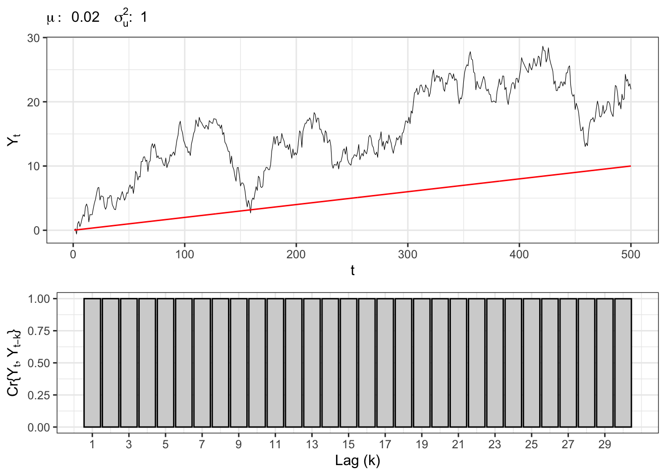
set.seed(1) # random seed# *************************************************# Inputs# *************************************************# Number of stepst_bar <-100000# Long term meanmu <-0.02# Variance residualssigma2_u <-1# *************************************************# Simulation# *************************************************# InitializationYt <-c(mu)# Simulated residualsu_t <-rnorm(t_bar, 0, sqrt(sigma2_u))# Simulated random-walk processfor(t in2:t_bar){ Yt[t] <- mu + Yt[t-1] + u_t[t]}
Figure 19.5: Random walk simulation and expected value (red) on the top. Empirical autocorrelation (gray).
Example: sampling from non-stationary AR(1)
Example 19.3 Let’s simulate a random walk process with drift with a Gaussian error, namely \(u_t \sim \mathcal{N}(0, \sigma_{\text{u}}^2)\).
Simulation of a non-stationary AR(1)
# *************************************************# Inputs# *************************************************set.seed(5) # random seedt_bar <-100# number of steps aheadj_bar <-2000# number of simulationssigma0 <-1# standard deviation of epsilonpar <-c(mu =0.3, phi1 =1) # parametersX0 <-c(0) # initial pointt_sample <-c(30,60,90) # sample times# *************************************************# Simulation# *************************************************# Process Simulationsscenarios <-tibble()for(j in1:j_bar){# Initialize X0 and standard deviation Xt <-rep(X0, t_bar) sigma <-rep(0, t_bar)# Simulated residuals eps <-rnorm(t_bar, mean=0, sd=sigma0)for(t in2:t_bar){ sigma[t] <- sigma0*sqrt(t-1) Xt[t] <- par[1] + par[2]*Xt[t-1] + eps[t] } df <-tibble(j =rep(j, t_bar), t =1:t_bar, Xt = Xt,sigma = sigma, eps = eps) scenarios <- dplyr::bind_rows(scenarios, df)}# Compute simulated momentsscenarios <- scenarios %>%group_by(t) %>%mutate(e_x =mean(Xt), sd_x =sd(Xt))# Trajectory jdf_j <- dplyr::filter(scenarios, j ==6)# Sample at different timesdf_t1 <- dplyr::filter(scenarios, t == t_sample[1])df_t2 <- dplyr::filter(scenarios, t == t_sample[2])df_t3 <- dplyr::filter(scenarios, t == t_sample[3])
Figure 19.6: Non-stationary AR(1) simulation with expected value (red), a possible trajectory (green) and samples for different times (blue) on the top. Theoretical (blue) and empirical (black) standard deviation at the bottom.
Sampling the process for different \(t\) we expect that, on a large number of simulations, the distribution will still be normal but with non-stationary moments, i.e. \[
Y_t \mid Y_0 \sim \mathcal{N}\left(Y_0 + \mu t, \sigma^{2}_u t \right) \text{.}
\] In the simulation below, the index \(t=1\) stores the initial value, so the number of innovations accumulated by the plotted observation is \(t-1\).
Figure 19.7: Non-stationary AR(1) histograms for different sampled times with normal pdf with empirical moments (blue) and normal pdf with theoretical moments (blue).
t
\[\mathbb{E}\{Y_t\}\]
\[\mathbb{E}^{\text{mc}}\{Y_t\}\]
\[\mathbb{V}\{Y_t\}\]
\[\mathbb{V}^{\text{mc}}\{Y_t\}\]
30
8.7
8.698311
29
29.69114
60
17.7
17.517805
59
60.09756
90
26.7
26.268452
89
90.05715
Table 19.6: Empirical and theoretical expectation, variance, covariance and correlation (first lag) for a non-stationary AR(1) process.
Wold, Herman. 1939. “A Study in the Analysis of Stationary Time Series. By Herman Wold.”Journal of the Institute of Actuaries 70 (1): 113–15. https://doi.org/10.1017/S0020268100011574.