In this section, we consider a sample of independent and identically distributed (IID) random variables. We recall that the notation \(\mathbf{x}_n = (x_1, \dots, x_i, \dots, x_n)\) denotes a possible realization of the random vector \(\mathbf{X}_n = (X_1, \dots, X_i, \dots, X_n)\), where the probability distribution of each \(X_i\) is equal to \(X_1\) for \(i = 1, \dots, n\).
10.1 Sample mean
The estimator of the sample expectation of an IID sample \(\mathbf{x}_n\) reads: \[
\hat{\mu}(\mathbf{x}_n) = \frac{1}{n}\sum_{i = 1}^{n} x_i
\text{.}
\tag{10.1}\]
Proposition 10.1 (Moments of the sample mean) If the random variables in the sample are IID, then the sample mean is an unbiased estimator of the expected value \(\mathbb{E}\{X_1\}\), i.e. \[
\mathbb{E}\left\{\hat{\mu}(\mathbf{X}_n) \right\} = \mathbb{E}\{X_1\}
\text{.}
\tag{10.2}\] In the same context, the variance of the sample mean estimator reads \[
\mathbb{V}\left\{\hat{\mu}(\mathbf{X}_n)\right\} = \frac{\mathbb{V}\{X_1\}}{n}
\text{.}
\tag{10.3}\]
Proof. If the random variables in the sample are IID, then all have the same expected value and variance, i.e. \(\mathbb{E}\{X_i\} = \mathbb{E}\{X_1\}\) and \(\mathbb{V}\{X_i\} = \mathbb{V}\{X_1\}\) for all \(i = 1, \dots, n\). Taking the expected value of the estimator in Equation 10.1 gives \[
\begin{aligned}
\mathbb{E}\left\{\hat{\mu}(\mathbf{X}_n) \right\} & {} = \frac{1}{n}\sum_{i = 1}^{n} \mathbb{E}\{X_i\} = && \text{(IID)} \\
& = \frac{1}{n} \sum_{i = 1}^{n} \mathbb{E}\left\{X_1\right\} = \\
& = \mathbb{E}\{X_1\}
\end{aligned}
\] Similarly, taking the variance of the sample mean estimator gives \[
\begin{aligned}
\mathbb{V}\left\{\hat{\mu}(\mathbf{X}_n)\right\} & {} = \frac{1}{n^2}\mathbb{V}\left\{\sum_{i = 1}^{n} X_i\right\} = && \text{(independence)} \\
& = \frac{1}{n^2} \sum_{i = 1}^{n} \mathbb{V}\left\{X_i\right\} = && \text{(identical distribution)} \\
& = \frac{1}{n^2} \sum_{i = 1}^{n} \mathbb{V}\left\{X_1\right\} = \\
& = \frac{\mathbb{V}\{X_1\}}{n}
\end{aligned}
\]
Proposition 10.2 (Distribution of the sample mean under IID) Under the IID assumption and with \(n\) sufficiently large, the central limit theorem (Theorem 8.1) applies. It states that, independently of the distribution of \(X_1\), the distribution of the sample mean converges to the distribution of a normal random variable, i.e. \[
\hat{\mu}(\mathbf{X}_n) \underset{n\to\infty}{\overset{\text{d}}{\longrightarrow}} \mathcal{N}\left(\mathbb{E}\{X_1\}, \frac{\mathbb{V}\{X_1\}}{n}\right)
\text{.}
\]
Proof. Let’s start the proof by considering the expectation and the variance of the following random variable, i.e. \[
S_n = \sum_{i = 1}^{n} X_i
\text{.}
\] The expectation and the variance of \(S_n\) can be easily obtained from Equation 10.2 and Equation 10.3 respectively and read: \[
\mathbb{E}\left\{S_n\right\} = n \cdot \mathbb{E}\{X_1\} \quad\quad \mathbb{V}\left\{S_n\right\} = n \cdot \mathbb{V}\{X_1\}
\] Applying the central limit theorem (Theorem 8.1), one obtains: \[
\frac{S_n - n \cdot \mathbb{E}\{X_1\}}{\sqrt{n} \cdot \mathbb{S}d\{X_1\}} = \frac{\frac{S_n}{n} - \mathbb{E}\{X_1\}}{\frac{\mathbb{S}d\{X_1\}}{\sqrt{n}}}
\underset{n\to\infty}{\overset{\text{d}}{\longrightarrow}}
\mathcal{N}(0, 1)
\text{.}
\] Thus, the random variable sample mean \(\hat{\mu}(\mathbf{X}_n) = \frac{S_n}{n}\) is distributed, on large samples, as a normal random variable, i.e. \[
\hat{\mu}(\mathbf{x}_n) = \frac{S_n}{n} = \frac{1}{n}\sum_{i = 1}^{n} x_i \underset{n \to \infty}{\overset{\text{d}}{\longrightarrow}} \mathcal{N}\left(\mathbb{E}\{X_1\}, \frac{\mathbb{V}\{X_1\}}{n}\right)
\text{.}
\]
Example: convergence in distribution of the sample mean
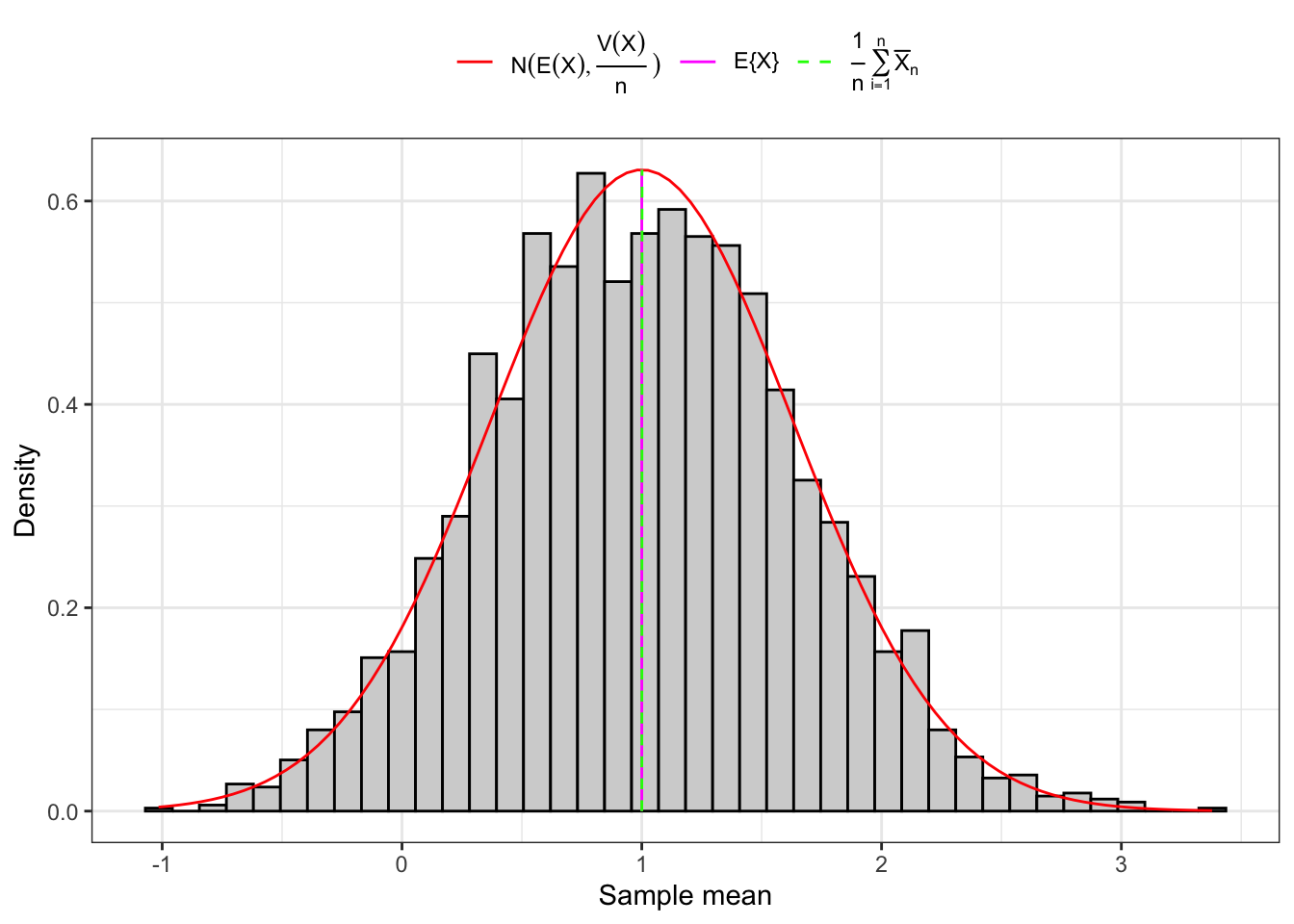
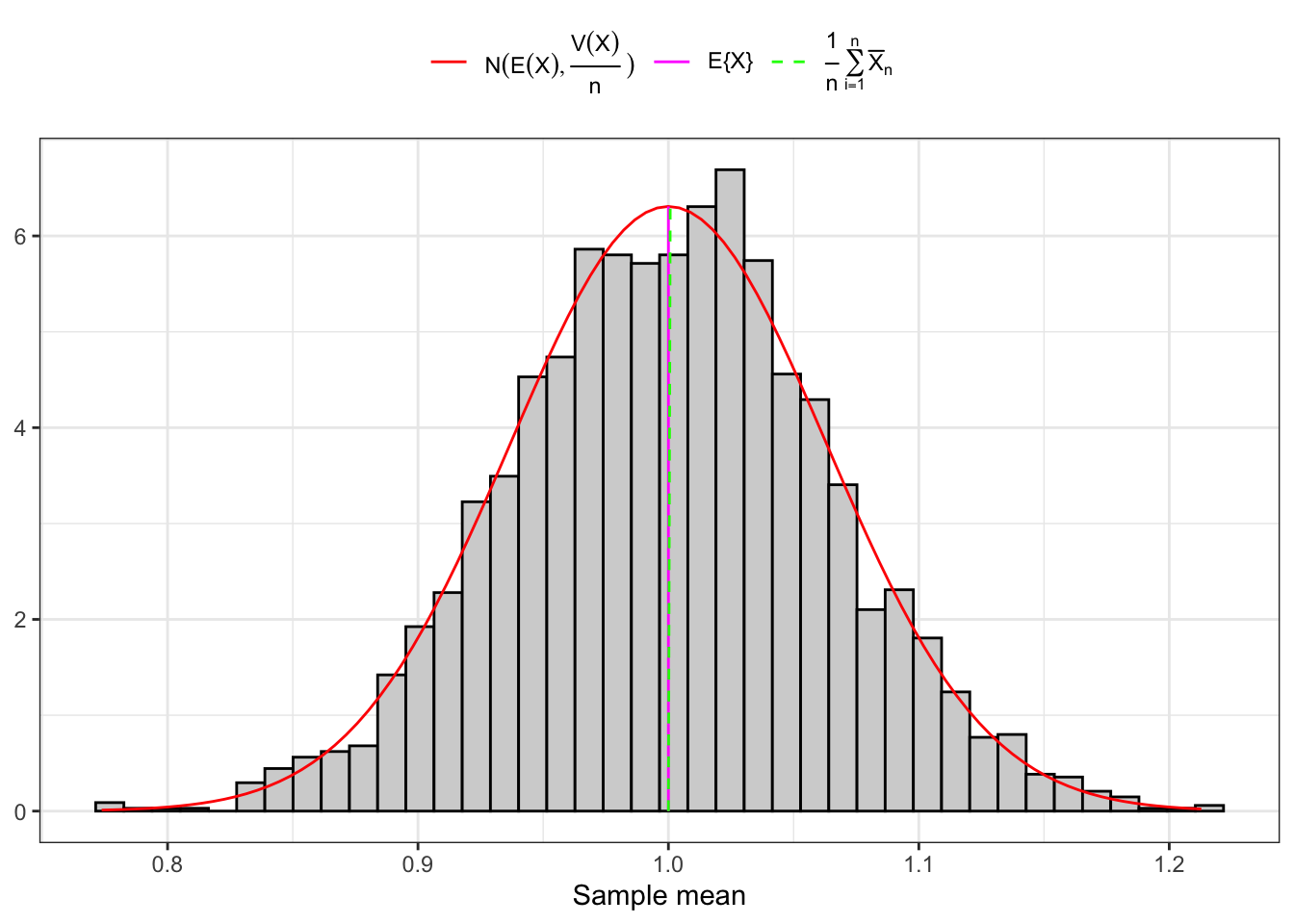
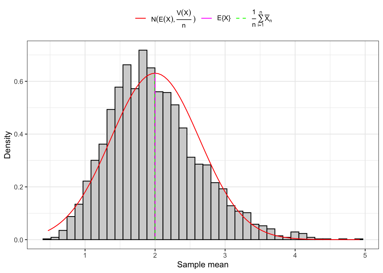
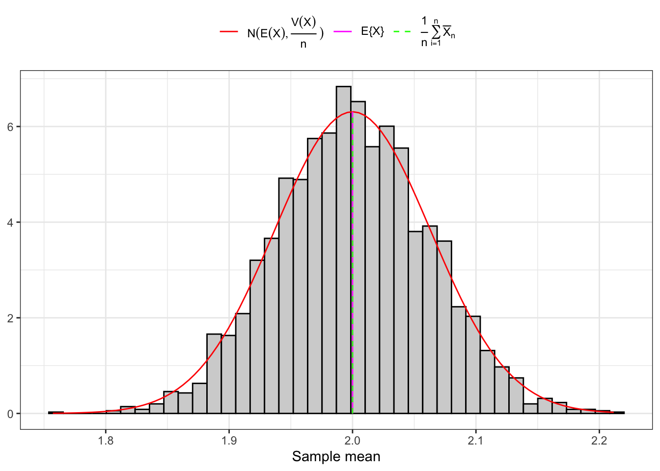
Example 10.1 As shown in Figure 10.1, convergence of the sample mean to a Normal random variable happens on large samples independently of the distribution of \(X_1\), but on small samples only if \(X_1\) is also normally distributed in the population. As shown in Figure 10.2, when \(X_1\) is, for example, Gamma distributed, convergence on small samples does not happen.
Distribution of sample mean of normal rv
# ================= Inputs =================# True population parameters (normal)true <-c(mu =1, sigma2 =4)# True Moments in populationmom <-c(mu = true[1], sigma2 = true[2])# Number of samplesn_sample <-3000# Number of observations for big samplesn <-1000# Number of observations for small samplesn_small <-10# ==========================================# Simulation of sample meanssample_small <- sample_large <-c()for(i in1:n_sample){set.seed(i)# Large sample x_large <-rnorm(n, true[1], sqrt(true[2]))# Small sample x_small <- x_large[1:n_small]# Sample mean sample_large[i] <-sum(x_large) / n sample_small[i] <-sum(x_small) / n_small}
(a) 3000 Small samples (10).
(b) 3000 Large samples (1000).
Figure 10.1: Distribution of the sample mean of IID Normal random variables.
Distribution of sample mean of Gamma distributed rv
# ================= Inputs =================# True population parameterstrue <-c(k =1, theta =2)# True Moments in population (Gamma rv)mom <-c(prod(true), true[1]*true[2]^2)# Number of samplesn_sample <-3000# Number of observations for big samplesn <-1000# Number of observations for small samplesn_small <-10# ==========================================# Simulation of sample meanssample_small <- sample_large <-c()for(i in1:n_sample){set.seed(i)# Large sample x_large <-rgamma(n, shape = true[1], scale = true[2])# Small sample x_small <- x_large[1:n_small]# Statistic on large sample sample_large[i] <-mean(x_large)# Statistic on small sample sample_small[i] <-mean(x_small)}
(a) 3000 Small samples (10).
(b) 3000 Large samples (1000).
Figure 10.2: Distribution of the sample mean of IID Gamma random variables.
10.2 Variance
The true population variance \(\sigma^2\) (Equation 5.10) of an IID sequence of random variables \(\mathbf{X}_n = (X_1, \dots, X_i, \dots, X_n)\) can be estimated on a sample \(\mathbf{x}_n = (x_1, \dots, x_i, \dots, x_n)\) with the sample’s variance estimator, i.e. \[
\hat{\sigma}^2(\mathbf{x}_n) = \frac{1}{n}\sum_{i = 1}^{n} \left[x_i - \hat{\mu}(\mathbf{x}_n)\right]^2
\text{.}
\tag{10.4}\] where \(\hat{\mu}\) is the estimator of the sample mean (Equation 10.1).
Equivalently, by applying property 2. of the variance (Equation 5.12) it can be estimated in terms of the first and second moments, i.e. \[
\begin{aligned}
\hat{\sigma}^2(\mathbf{x}_n) & {} = \hat{\mu}(\mathbf{x}_n^2) - \hat{\mu}(\mathbf{x}_n)^2 = \\
& =
\frac{1}{n}\sum_{i = 1}^{n} x_i^2 - \left(\frac{1}{n}\sum_{i = 1}^{n} x_i\right)^2
\text{.}
\end{aligned}
\tag{10.5}\]
Proposition 10.3 (Moments of the sample variance) The sample’s variance defined in Equation 10.4 - Equation 10.5 is a biased estimator of the true variance in population \(\sigma^2 = \mathbb{V}\{X_1\}\), i.e. \[
\mathbb{E}\left\{\hat{\sigma}^2(\mathbf{X}_n) \right\} = \frac{n-1}{n} \sigma^2
\text{,}
\] with a bias that disappears on large samples as \(n \to \infty\).
A correct estimator of the population variance is the corrected sample’s variance, i.e. \[
\hat{s}^2(\mathbf{x}_n) = \frac{n}{n-1} \hat{\sigma}^2(\mathbf{x}_n)
\text{,}
\tag{10.6}\] that satisfies \[
\mathbb{E}\left\{\hat{s}(\mathbf{X}_n) \right\} = \mathbb{V}\{X_1\}
\text{.}
\tag{10.7}\] In the same context, the variance of the corrected sample variance estimator reads \[
\mathbb{V}\left\{\hat{s}^2(\mathbf{X}_n)\right\} = \frac{\sigma^4}{n}\left(\frac{\mu_4}{\sigma^4}-1 + \frac{2}{n-1}\right)
\text{,}
\tag{10.8}\] where \(\frac{\mu_4}{\sigma^4}\) is the kurtosis (Equation 5.19) of \(\mathbf{X}_n\).
Example: moments of the corrected sample variance
Example 10.2 Let’s consider 20000 IID samples extracted from Gamma random variables with parameters \(k = 1\) and \(\theta = 2\). Notably, the expectation and variance of a Gamma distributed random variable read: \[
\mathbb{E}\{X\} = k \cdot \theta \text{,} \quad \mathbb{V}\{X\} = k \cdot \theta^2
\text{,}
\] while the skewness and kurtosis read \[
\mathbb{S}k\{X\} = \frac{2}{\sqrt{k}} \text{,} \quad \mathbb{K}t\{X\} = \frac{6}{k}+3
\text{.}
\] Let’s estimate the expectation and variance of the sample variance and the corrected sample variance considering samples with \(n_{\text{small}} = 40\) and \(n_{\text{large}} = 1000\).
Moments of corrected sample variance
# ================= Inputs =================# True population parameters (Gamma rv)true <-c(k =1, theta =2)# True population moments (Gamma rv)mom <-c(mu = true[["k"]]*true[["theta"]],sigma2 = true[["k"]]*true[["theta"]]^2,sk =2/sqrt(true[["k"]]),kt =6/ true[["k"]] +3)# Number of elements for large samplesn <-1000# Number of elements for small samplesn_small <-40# Number of samplesn_sample <-20000# ==========================================# Simulation of sample variancesample_small <- sample_large <-c()sample_small_c <- sample_large_c <-c()for(i in1:n_sample){set.seed(i)# Large sample x_large <-rgamma(n, shape = true[1], scale = true[2])# Small sample x_small <- x_large[1:n_small]# Sample variance sample_large[i] <- (1/n)*sum((x_large -mean(x_large))^2) sample_small[i] <- (1/n_small)*sum((x_small -mean(x_small))^2)# Corrected sample variance sample_large_c[i] <- (n/(n-1)) * sample_large[i] sample_small_c[i] <- (n_small/(n_small-1)) * sample_small[i]}# True variance of the correct sample variance by formulastrue_var <-c(mom[2]^2/n_small * (mom[4] -1+2/(n_small-1)), mom[2]^2/n * (mom[4] -1+2/(n-1)))
n
\(\sigma^2\)
\(\mathbb{E}\{\hat{\sigma}^2\}\)
\(\mathbb{E}\{\hat{s}^2\}\)
\(\mathbb{V}\{s^2\}\)
\(\mathbb{V}\{\hat{\sigma}^2\}\)
\(\mathbb{V}\{\hat{s}^2\}\)
40
4
3.872863
3.972167
3.220513
3.0403443
3.1982583
1000
4
3.993620
3.997618
0.128032
0.1263861
0.1266393
Table 10.1: Moments of the sample variance and corrected sample variance.
Proposition 10.4 (Distribution of the corrected sample variance under normality) Under the assumption of an IID normal sample, \(\frac{\mu_4}{\sigma^4} = 3\) and the variance simplifies to: \[
\mathbb{V}\left\{\hat{s}^2(\mathbf{X}_n)\right\} = \frac{2\sigma^4}{n-1}
\text{.}
\tag{10.9}\] Moreover, from Cochran’s theorem the statistic \[
T(\mathbf{X}_n) = (n-1)\frac{\hat{s}^2(\mathbf{X}_n)}{\sigma^2} \sim \chi^2(n-1)
\text{.}
\tag{10.10}\] Going to the limit as \(n \to \infty\) a \(\chi^2(n)\) random variable converges to a standard normal random variable (see Section 32.1.1), i.e. \[
\frac{\chi^2(n) - n}{\sqrt{2n}} \underset{n\to\infty}{\overset{\text{d}}{\longrightarrow}} \mathcal{N}(0,1)
\text{,}
\] therefore, on large samples the statistic converges to a normal random variable, i.e. \[
T(\mathbf{X}_n) \underset{n\to\infty}{\overset{\text{d}}{\longrightarrow}} \mathcal{N}(n,2n)
\text{.}
\tag{10.11}\]
If the population \(\mathbf{X}_n\) are IID normally distributed, then the distribution of \(\hat{s}^2(\mathbf{X}_n)\) is proportional to the distribution of a \(\chi^2(n-1)\). In fact, from Equation 10.10 the expectation of \(\hat{s}^2(\mathbf{X}_n)\) reads \[
\begin{aligned}
\mathbb{E}\{T(\mathbf{X}_n)\} & {} = (n-1)\frac{\mathbb{E}\{\hat{s}^2(\mathbf{X}_n)\}}{\sigma^2} \\
& \implies \mathbb{E}\{\hat{s}^2(\mathbf{X}_n)\} = \frac{\sigma^2 \mathbb{E}\{T(\mathbf{X}_n)\}}{n-1} = \frac{\sigma^2 (n-1)}{n-1} = \sigma^2
\end{aligned}
\] Similarly, computing the variance of Equation 10.10 and knowing that \(\mathbb{V}\{T(\mathbf{X}_n)\} = 2(n-1)\), one obtains: \[
\begin{aligned}
\mathbb{V}\{T(\mathbf{X}_n)\} & {} = (n-1)^2\frac{\mathbb{V}\{\hat{s}^2(\mathbf{X}_n)\}}{\sigma^4} \\
& \implies \mathbb{V}\{\hat{s}^2(\mathbf{X}_n)\} = \frac{\sigma^4 \mathbb{V}\{T(\mathbf{X}_n)\}}{(n-1)^2} = \frac{\sigma^4 2 (n-1)}{(n-1)^2} = \frac{2\sigma^4}{n-1}
\end{aligned}
\]
Example: Distribution of the corrected sample variance under normality
Example 10.3 Let’s consider 3000 IID samples extracted from Normal random variables with parameters \(\mu = 1\) and \(\sigma^2 = 4\). Notably, the skewness and kurtosis read \[
\mathbb{S}k\{X\} = 0 \text{,} \quad \mathbb{K}t\{X\} = 3
\text{.}
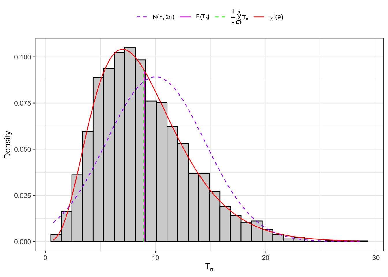
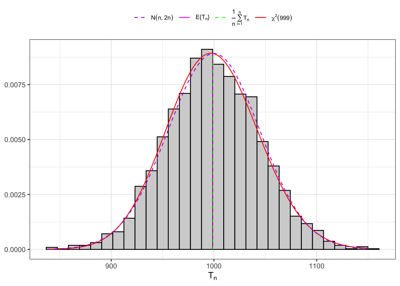
\] Let’s evaluate the distribution of the corrected sample variance (Equation 10.10) and the asymptotic distribution (Equation 10.11) of the statistic \(T(\mathbf{X}_n)\) from Proposition 10.4.
Distribution of corrected sample variance under normality.
# ================= Inputs =================# True population parameterstrue <-c(mu =1, sigma2 =4)# True Moments in population (Gamma rv)mom <-c(true)# Number of samplesn_sample <-3000# Number of observations for big samplesn <-1000# Number of observations for small samplesn_small <-10# ==========================================# Simulation of sample variancesample_small <- sample_large <-c()for(i in1:n_sample){set.seed(i)# Large sample x_large <-rnorm(n, true[1], sqrt(true[2]))# Small sample x_small <- x_large[1:n_small]# Sample mean mu_hat_large <- (1/n)*sum(x_large) mu_hat_small <- (1/n_small)*sum(x_small)# Corrected sample variance sample_large[i] <- (1/(n-1)) *sum((x_large - mu_hat_large)^2) sample_small[i] <- (1/(n_small-1)) *sum((x_small - mu_hat_small)^2)}
(a) Small sample (166).
(b) Large sample (5000).
Figure 10.3: Distribution of the statistic \(T_n\) under normality.
10.3 Skewness
Let’s consider an IID sample \(\mathbf{x}_n = (x_1, \dots, x_i, \dots, x_n)\), then the sample’s skewness is an estimator of the form: \[
b_1(\mathbf{x}_n) = \frac{1}{n}\sum_{i = 1}^{n} \left(\frac{x_i - \hat{\mu}(\mathbf{x}_n)}{\sqrt{\hat{\sigma}^2(\mathbf{x}_n)}}\right)^3
\text{.}
\tag{10.12}\] The estimator in Equation 10.12 is not correct for the true population skewness (Equation 5.18). A correct estimator of the skewness reads: \[
g_1(\mathbf{x}_n) = \frac{\sqrt{n(n-1)}}{(n-2)} b_1(\mathbf{x}_n)
\text{.}
\tag{10.13}\]
Proposition 10.5 (Distribution of the sample skewness under normality) Under the assumption of an IID normal sample, the asymptotic moments of the sample skewness are: \[
\mathbb{E}\{b_1(\mathbf{X}_n)\} = 0 \text{,} \quad \mathbb{V}\{b_1(\mathbf{X}_n)\} = \frac{6}{n}
\text{.}
\] Notably, from Urzúa (1996) the exact mean of the estimator in Equation 10.12 corrected for small samples reads \[
\mathbb{E}\{b_1(\mathbf{X}_n)\} = 0
\text{,}
\] and variance \[
\mathbb{V}\{b_1(\mathbf{X}_n)\} = \frac{6(n-2)}{(n+1)(n+3)}
\text{.}
\tag{10.14}\] Thus, under normality, the asymptotic distribution of the sample skewness is normal i.e. \[
b_1(\mathbf{X}_n) \underset{n \to \infty}{\overset{\text{d}}{\longrightarrow}} \mathcal{N}\left(0, \frac{6}{n} \right)
\text{.}
\tag{10.15}\]
Example: Distribution of the corrected sample skewness under normality
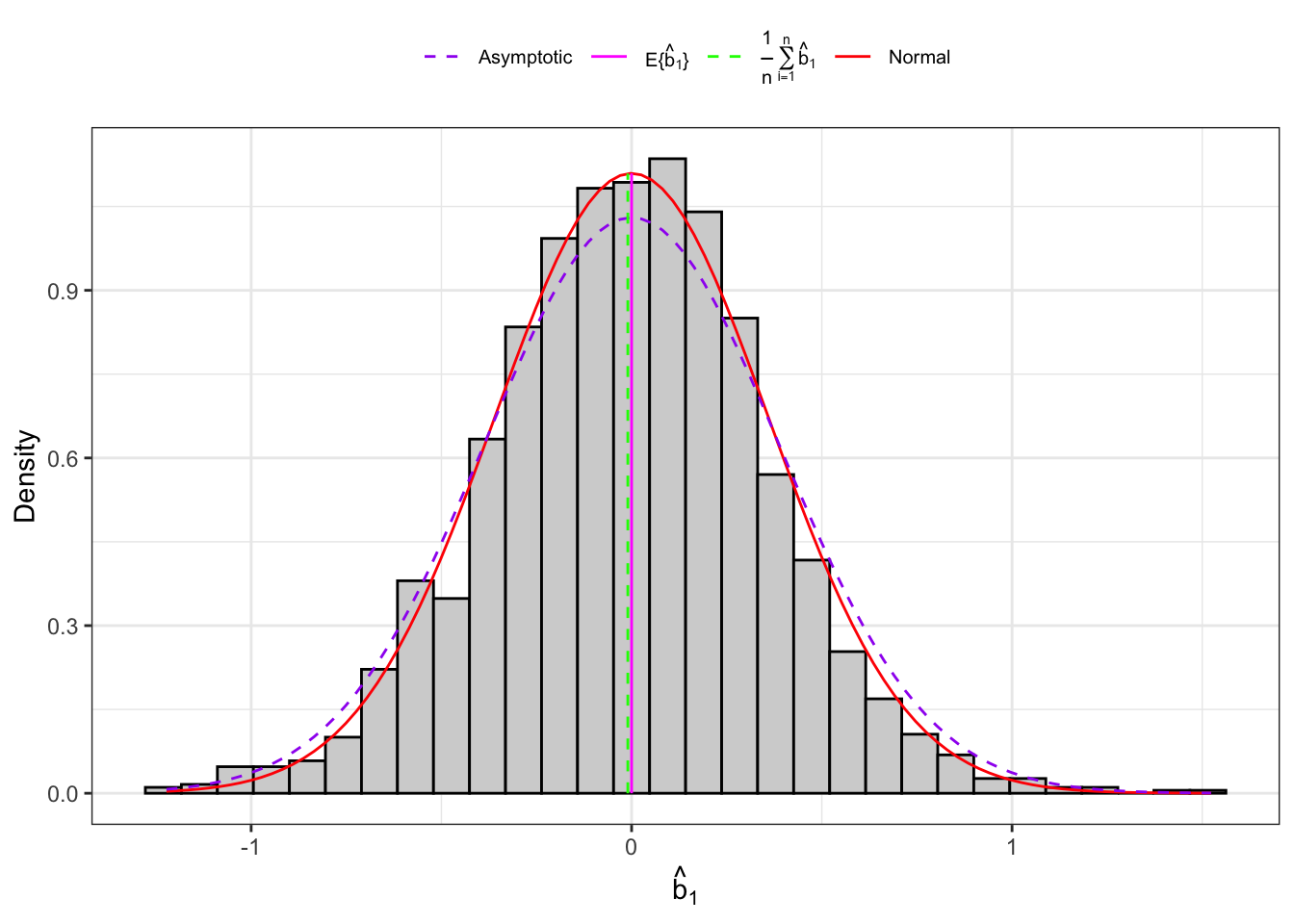
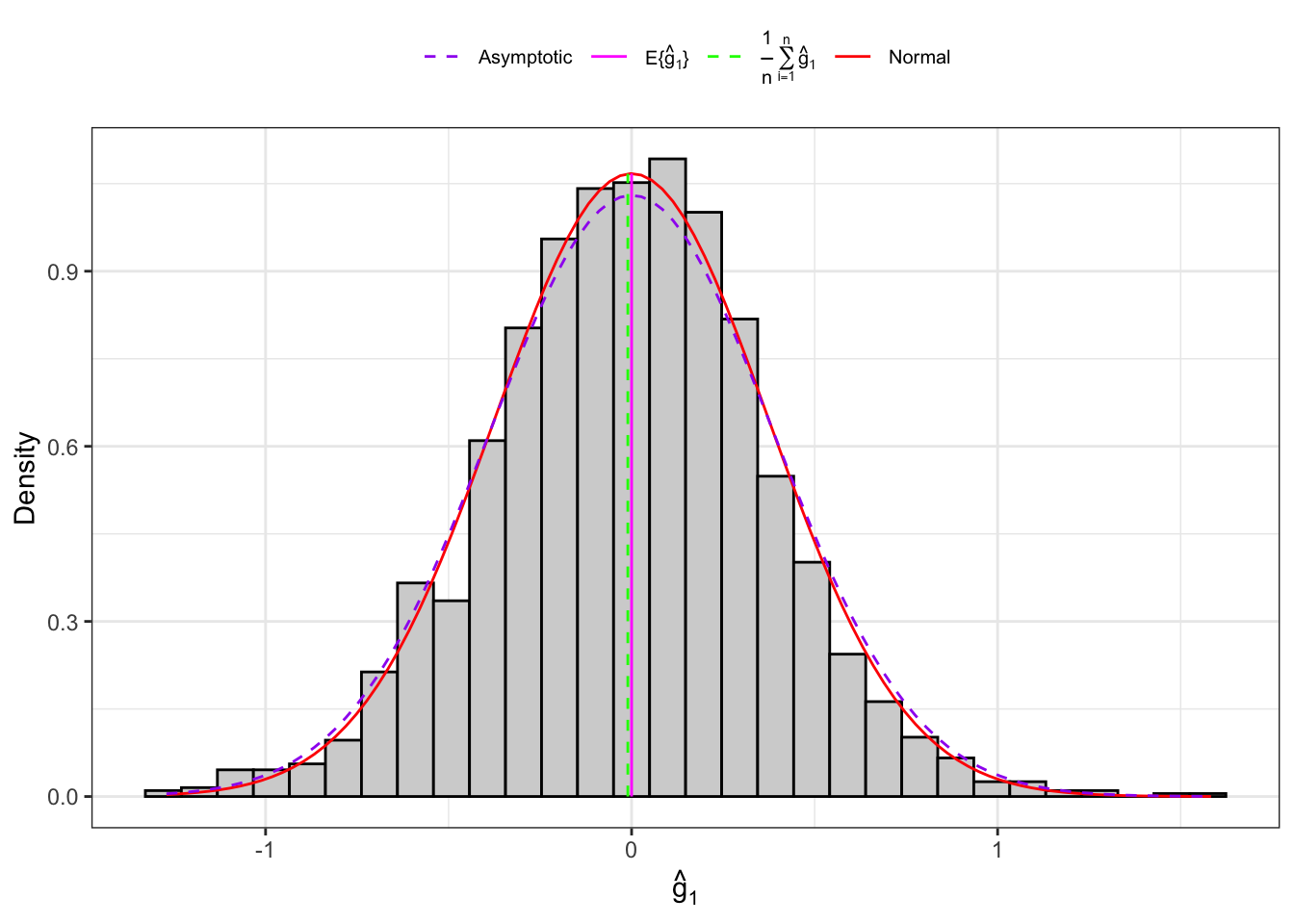
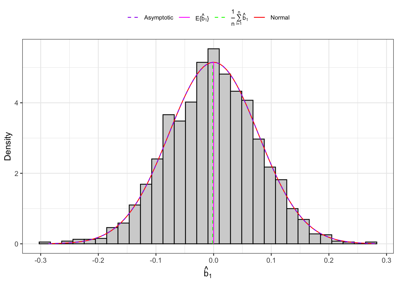
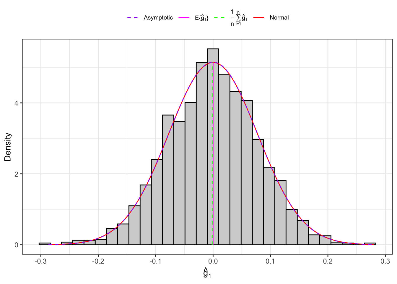
Example 10.4 Let’s consider an IID normal sample, \(\mathbf{X}_n = (X_1, \dots, X_n)\) and let’s simulate 2000 IID samples. Then, for each sample we compute the sample skewness as defined in Equation 10.12 and Equation 10.13 and their theoretical moments as defined in Proposition 10.5.
Distribution of sample skewness under normality.
# ================= Inputs =================set.seed(1)# True population parameterstrue <-c(mu =1, sigma2 =4)# True population moments (Gamma rv)mom <-c(true, sk =0, kt =3)# Number of elements for large samplesn <-1000# Number of elements for small samplesn_small <-40# Number of samplesn_sample <-2000# ==========================================# Simulation of sample variancesample_small <- sample_large <-c()sample_small_c <- sample_large_c <-c()for(i in1:n_sample){set.seed(i)# Large sample x_large <-rnorm(n, mean = true[1], sd =sqrt(true[2]))# Small sample x_small <-rnorm(n_small, mean = true[1], sd =sqrt(true[2]))# Sample mean mu_hat_large <- (1/n)*sum(x_large) mu_hat_small <- (1/n_small)*sum(x_small)# Sample variance sigma2_hat_large <- (1/n) *sum((x_large - mu_hat_large)^2) sigma2_hat_small <- (1/n_small) *sum((x_small - mu_hat_small)^2)# Sample skewness sample_large[i] <- (1/n)*sum(((x_large - mu_hat_large)/sqrt(sigma2_hat_large))^3) sample_small[i] <- (1/n_small)*sum(((x_small - mu_hat_small)/sqrt(sigma2_hat_small))^3)# Corrected Sample skewness sample_large_c[i] <-sqrt(n*(n-1))/(n-2) * sample_large[i] sample_small_c[i] <-sqrt(n_small*(n_small-1))/(n_small-2) * sample_small[i]}# True variance of the correct sample variance by formulastrue_var_b1 <-c(6* (n_small -2) / ((n_small +1) * (n_small +3)), 6/ n)true_var_g1 <- true_var_b1 *c(n_small * (n_small -1) / (n_small -2)^2, n * (n -1) / (n -2)^2)
n
\(b_1\)
\(\mathbb{E}\{\hat{b}_1\}\)
\(\mathbb{E}\{\hat{g}_1\}\)
\(\mathbb{V}\{b_1\}\)
\(\mathbb{V}\{g_1\}\)
\(\mathbb{V}\{\hat{b}_1\}\)
\(\mathbb{V}\{\hat{g}_1\}\)
40
0
-0.0099361
-0.0103275
0.129325
0.139714
0.1307748
0.1412802
1000
0
-0.0015675
-0.0015699
0.006000
0.006018
0.0061388
0.0061572
Table 10.2: Moments of the sample skewness and corrected sample skewness
(a) Small samples.
(b) Small samples.
(c) Large samples.
(d) Large samples.
Figure 10.4: Distribution of the skewness under normality.
10.4 Kurtosis
Let’s consider an IID sample \(\mathbf{x}_n = (x_1, \dots, x_i, \dots, x_n)\); then the population kurtosis (Equation 5.19) is estimated as follows: \[
b_2(\mathbf{x}_n) = \frac{1}{n}\sum_{i = 1}^{n} \left(\frac{x_i - \hat{\mu}(\mathbf{x}_n)}{\sqrt{\hat{\sigma}^2(\mathbf{x}_n)}}\right)^4
\text{.}
\tag{10.16}\] The estimator in Equation 10.16 is not correct. From Pearson (1931), a corrected version of \(b_2(\mathbf{x}_n)\) is defined as: \[
g_2(\mathbf{x}_n) = \left[b_2(\mathbf{x}_n) - \frac{3(n+1)}{n+1} \right]\frac{(n+1)(n-1)}{(n-2)(n-3)}
\text{.}
\tag{10.17}\]
Proposition 10.6 (Distribution of the sample kurtosis under normality) Under the assumption of an IID normal sample, the asymptotic moments of the sample kurtosis are: \[
\mathbb{E}\{b_2(\mathbf{X}_n)\} = 3 \text{,} \quad \mathbb{V}\{b_2(\mathbf{X}_n)\} = \frac{24}{n}
\text{.}
\] Notably, Urzúa (1996) also reports the exact mean and variance for a small normal sample, i.e. \[
\mathbb{E}\{b_2(\mathbf{X}_n)\} = \frac{3(n-1)}{(n+1)}
\text{,}
\tag{10.18}\] and the variance as: \[
\mathbb{V}\{b_2(\mathbf{X}_n)\} = \frac{24n(n-2)(n-3)}{(n+1)^2(n+3)(n+5)}
\text{.}
\tag{10.19}\] Thus, under normality, the asymptotic distribution of the sample kurtosis is normal, i.e. \[
b_2(\mathbf{X}_n) \underset{n \to \infty}{\overset{\text{d}}{\longrightarrow}} \mathcal{N}\left(3, \frac{24}{n} \right)
\text{.}
\tag{10.20}\]
Example: Distribution of the corrected sample kurtosis under normality
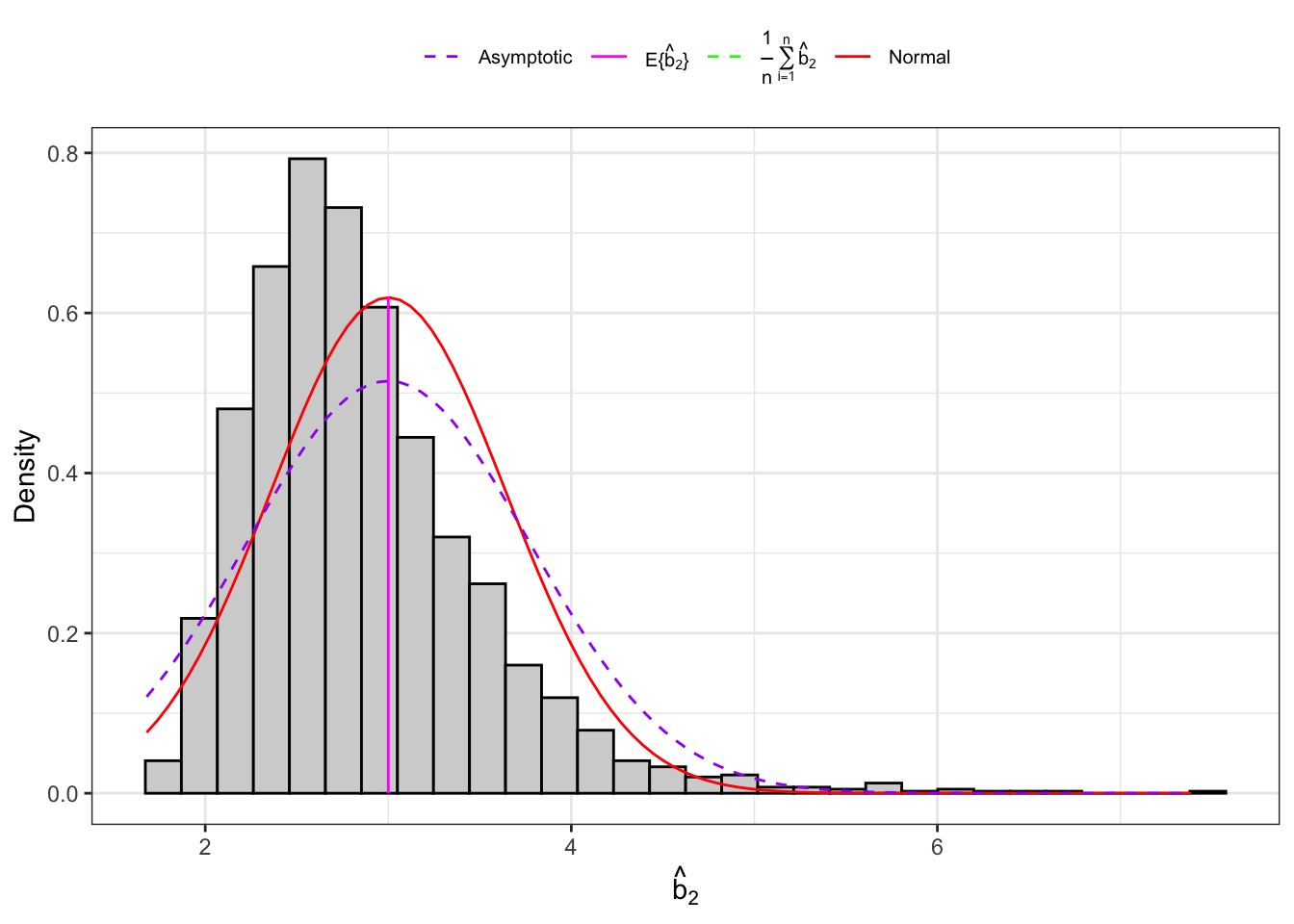
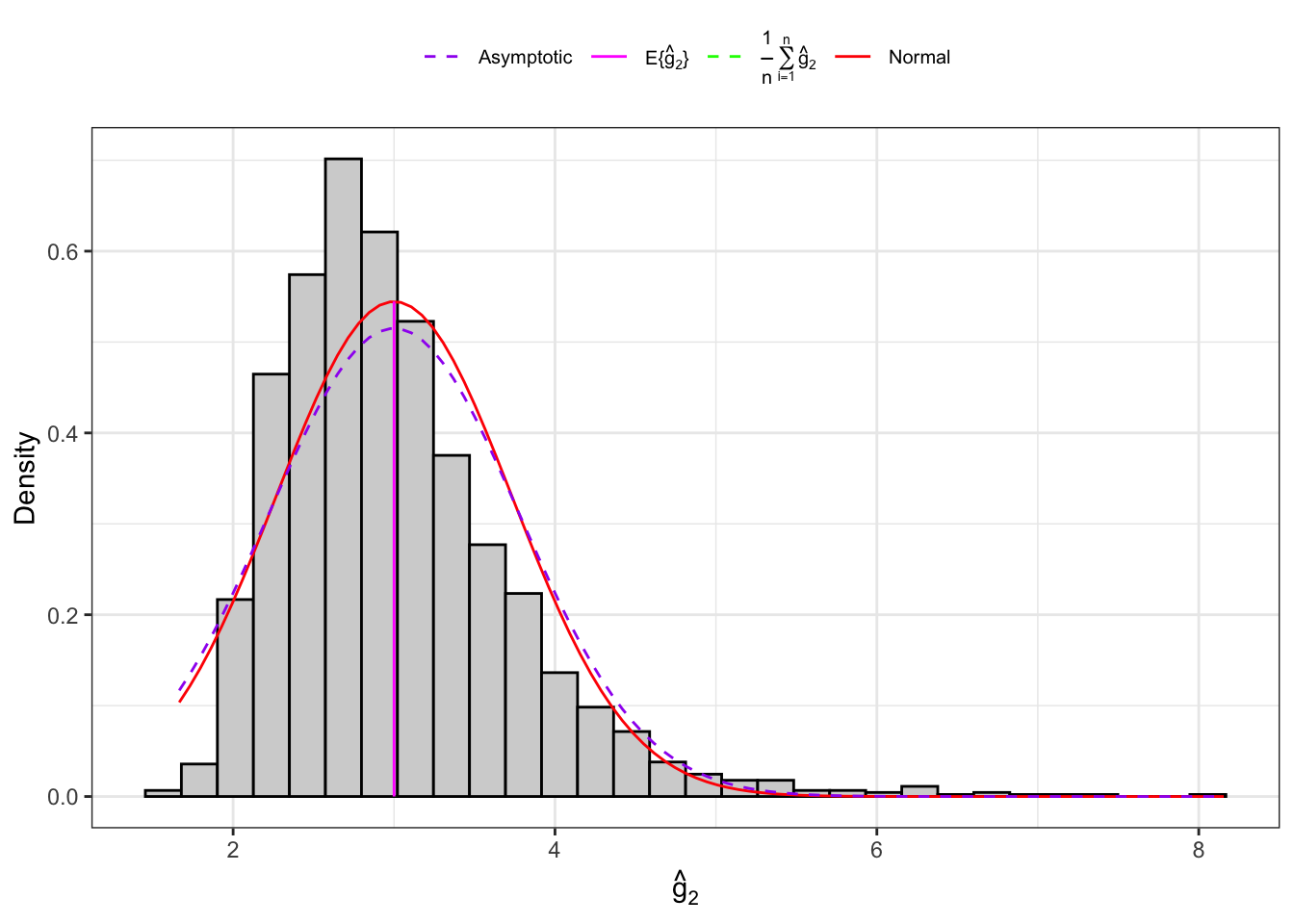
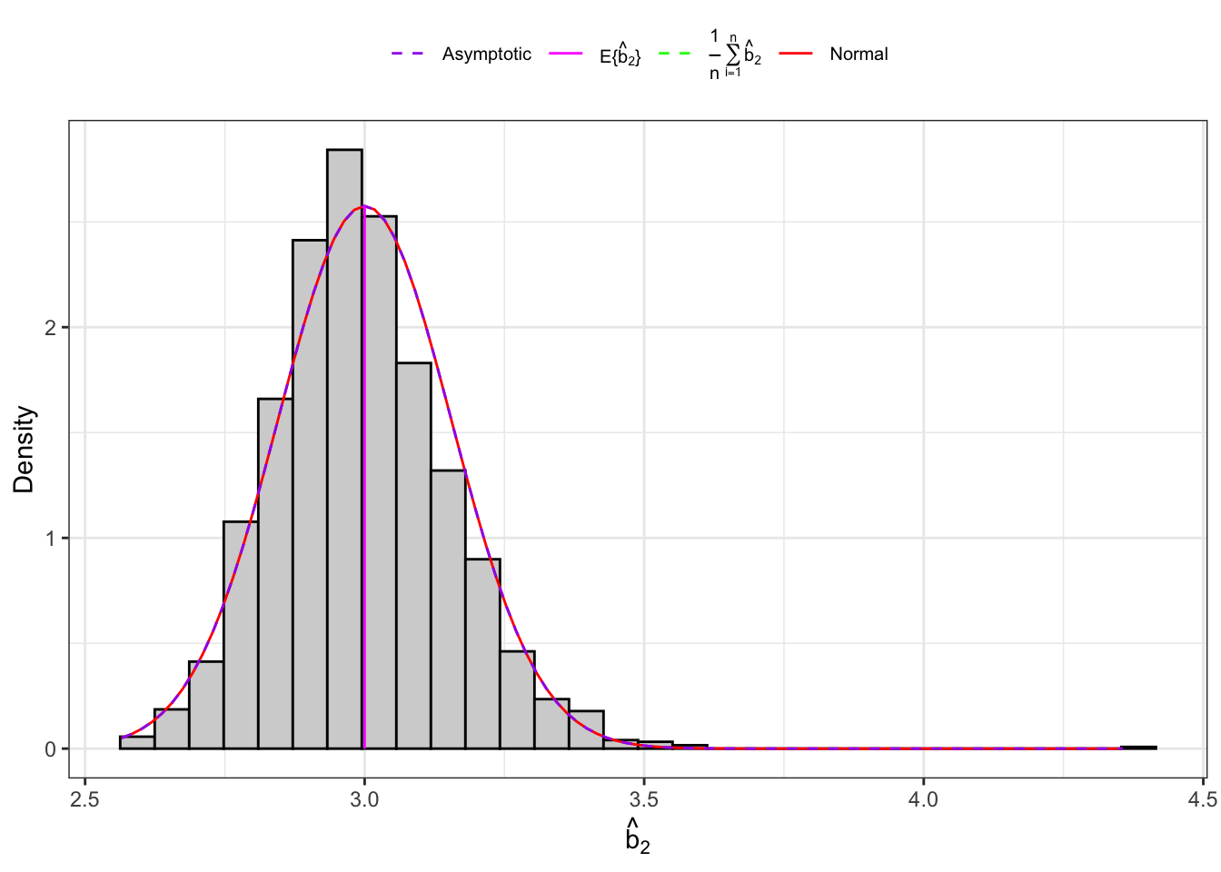
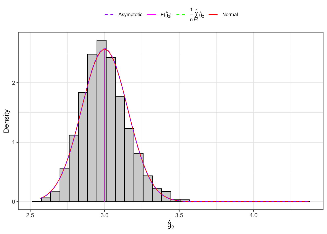
Example 10.5 Let’s consider an IID normal sample, \(\mathbf{X}_n = (X_1, \dots, X_n)\) and let’s simulate 2000 IID samples. Then, for each sample we compute the sample kurtosis as defined in Equation 10.16 and Equation 10.17 and their theoretical moments as defined in Proposition 10.6.
Distribution of sample kurtosis under normality.
# ================= Inputs =================set.seed(1)# True population parameterstrue <-c(mu =1, sigma2 =4)# True population moments (Gamma rv)mom <-c(true, sk =0, kt =3)# Number of elements for large samplesn <-1000# Number of elements for small samplesn_small <-40# Number of samplesn_sample <-2000# ==========================================# Simulation of sample variancesample_small <- sample_large <-c()sample_small_c <- sample_large_c <-c()for(i in1:n_sample){set.seed(i)# Large sample x_large <-rnorm(n, mean = true[1], sd =sqrt(true[2]))# Small sample x_small <-rnorm(n_small, mean = true[1], sd =sqrt(true[2]))# Sample mean mu_hat_large <- (1/n)*sum(x_large) mu_hat_small <- (1/n_small)*sum(x_small)# Sample variance sigma2_hat_large <- (1/n) *sum((x_large - mu_hat_large)^2) sigma2_hat_small <- (1/n_small) *sum((x_small - mu_hat_small)^2)# Sample skewness sample_large[i] <- (1/n)*sum(((x_large - mu_hat_large)/sqrt(sigma2_hat_large))^4) sample_small[i] <- (1/n_small)*sum(((x_small - mu_hat_small)/sqrt(sigma2_hat_small))^4)# Corrected Sample skewness sample_large_c[i] <- (sample_large[i] -3*(n-1)/(n+1) ) * (n+1) * (n-1) / ((n-2)*(n-3)) +3 sample_small_c[i] <- (sample_small[i] -3*(n_small-1)/(n_small+1) ) * (n_small+1) * (n_small-1) / ((n_small-2)*(n_small-3)) +3}# True variance of the correct sample variance by formulastrue_var_b2 <-c(24* n_small * (n_small -2) * (n_small -3) / ((n_small +1)^2* (n_small +3) * (n_small +5)), 24/ n)true_var_g2 <- true_var_b2 *c((n_small+1) * (n_small-1) / ((n_small-2)*(n_small-3)), (n+1) * (n-1) / ((n-2)*(n-3)))^2
n
\(b_2\)
\(\mathbb{E}\{\hat{b}_2\}\)
\(\mathbb{E}\{\hat{g}_2\}\)
\(\mathbb{V}\{b_2\}\)
\(\mathbb{V}\{g_2\}\)
\(\mathbb{V}\{\hat{b}_2\}\)
\(\mathbb{V}\{\hat{g}_2\}\)
40
3
2.862257
3.009779
0.4149616
0.5367032
0.4178224
0.5404034
1000
3
2.993902
2.999896
0.0240000
0.0242415
0.0242128
0.0244565
Table 10.3: Moments of the sample kurtosis and corrected sample kurtosis
(a) Small samples.
(b) Small samples.
(c) Large samples.
(d) Large samples.
Figure 10.5: Distribution of the kurtosis under normality.