26 Value at Risk test
The Value at Risk (VaR) of a random variable \(X\) is a measure of risk that represents the lower-tail threshold exceeded with probability \(\alpha\). Formally, \[ \mathbb{P}(X \le \text{VaR}^{\alpha}(X)) = \alpha \text{.} \] If the random variable \(X\) has known distribution \(F_X\) and quantile function \(q_X\), the Value at Risk is defined as \[ \text{VaR}^{\alpha}(X) = q_X(\alpha) \text{,} \] where \(q_X\) is the quantile function of \(X\).
Value at Risk
#' @param q_X Quantile function of X.
#' @param alpha Probability
VaR <- function(q_X, alpha){
  q_X(alpha)
}
# Confidence level
alpha <- 0.05
# Quantile functions
q_X1 <- function(p) qnorm(p)
q_X2 <- function(p) qlogis(p)
q_X3 <- function(p) qt(p, df = 5)
# VaR
VaR_X1 <- VaR(q_X1, alpha)
VaR_X2 <- VaR(q_X2, alpha)
VaR_X3 <- VaR(q_X3, alpha)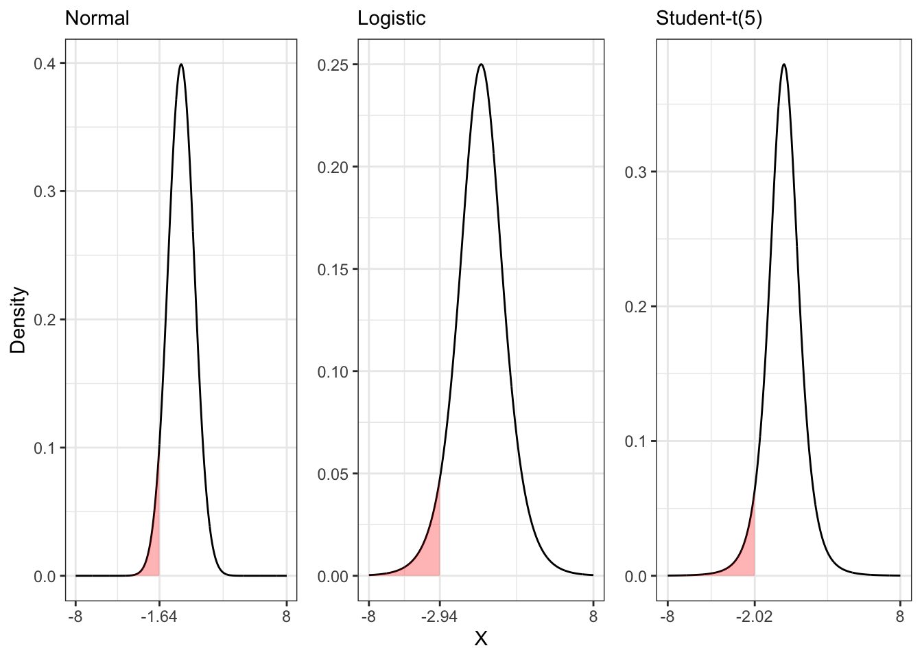
Another important measure of risk is the Expected Shortfall (ES) that, given a certain level \(\alpha\), represents the average of the lower-tail quantiles up to \(\alpha\). More precisely, \[ \text{ES}^{\alpha}(X) = \frac{1}{\alpha} \int_{0}^{\alpha} \text{VaR}^{\gamma}(X) d\gamma \] The Expected Shortfall is also called conditional value at risk (CVaR) or superquantile.
| Distribution | \(\alpha\) | \(\text{VaR}^{\alpha}(X)\) | \(\text{ES}^{\alpha}(X)\) |
|---|---|---|---|
| Normal | 0.05 | -1.644854 | -2.062713 |
| Student-t | 0.05 | -2.015048 | -2.890129 |
| Logistic | 0.05 | -2.944439 | -3.970305 |
Example 26.1 Let’s consider a process \(Y_t\) following an ARMA(2,2)-GARCH(1,1), i.e. \[ \begin{aligned} & {} Y_t = \mu + \phi_1 Y_{t-1} + \phi_2 Y_{t-2} + \theta_1 e_{t-1} + \theta_2 e_{t-2} + e_t \\ & e_t = \sigma_t u_t \\ & \sigma_t^2 = \omega + \alpha_1 e_{t-1}^{2} + \beta_1 \sigma_{t-1}^{2} \end{aligned} \] with \(u_t \sim \mathcal{N}(0,1)\). The conditional expectation \(\mathbb{E}\{Y_t \mid \mathcal{F}_{t-1}\}\) is equal to \[ \mu_t = \mu + \phi_1 Y_{t-1} + \phi_2 Y_{t-2} + \theta_1 e_{t-1} + \theta_2 e_{t-2} \] while the conditional variance is \[ \mathbb{V}\{Y_t \mid \mathcal{F}_{t-1}\} = \sigma_t^2 \] Since \(u_t\) is normally distributed, the conditional distribution of \(Y_t\) given \(\mathcal{F}_{t-1}\) is also normal, i.e. \[ Y_{t \mid t-1} \sim \mathcal{N}(\mu_t, \sigma^2_t) \] Therefore, the conditional Value at Risk (VaR) with lower-tail probability \(\alpha\) is \[ \text{VaR}_{t \mid t-1}^{\alpha} = \mu_t + \sqrt{\sigma^2_t} q(\alpha) \] where \(q(\alpha)\) is the quantile with probability \(\alpha\) of a standard normal.
26.1 Test on the number of violations
Let’s define a violation of the conditional VaR with level \(\alpha\) as \[ V_t = \mathbb{1}_{[Y_t \le \text{VaR}_{t \mid t-1}^{\alpha}]} \] The violation indicator \(V_t\) is Bernoulli distributed, i.e. \[ V_t \sim \text{Bernoulli}(\alpha) \text{,} \] with mean and variance equal to \[ \mathbb{E}\{V_t\} = \alpha \text{,}\quad \mathbb{V}\{V_t\} = \alpha (1-\alpha) \]
26.1.1 Asymptotic variance
If the violation indicators are IID, then we can standardize \(V_t\) and apply the central limit theorem (CLT) to obtain that \[ \text{T}_1^{\alpha} = \frac{1}{\sqrt{n}} \sum_{i = 1}^{n} \left(\frac{V_i - \alpha}{\sqrt{\alpha(1-\alpha)}} \right) \underset{n\to\infty}{\overset{\text{d}}{\longrightarrow}} \mathcal{N}(0, 1) \text{,} \] converges in distribution to a standard normal. Under the null hypothesis \(\mathcal{H}_0\), i.e. \[ \mathcal{H}_0: \mathbb{P}\{Y_t \le \text{VaR}_{t|t-1}^{\alpha}\} = \alpha \] that is equivalent to saying that the VaR is correctly specified, we reject \(\mathcal{H}_0\) if \[ \mathcal{H}_0 \text{ is rejected} \iff \text{T}_1^{\alpha} < q_{\alpha/2} \text{,}\quad\text{OR}\quad \text{T}_1^{\alpha} > |q_{\alpha/2}| \] where \(q_{\alpha}\) is the quantile with level \(\alpha \in (0,1)\) of a standard normal.
26.1.2 Empirical variance
Let’s define the total number of violations of the conditional VaR as \[ S_n = \sum_{i = 1}^{n} V_i \text{,} \] and let’s use it to estimate the empirical variance of the number of violations. Instead of using the theoretical variance \(\alpha(1-\alpha)\), let’s compute \[ \alpha(1-\alpha) \longrightarrow \frac{S_n}{n} \left(1 - \frac{S_n}{n} \right) \text{.} \] Hence, we obtain a new statistic \[ \text{T}_2^{\alpha} = \frac{1}{\sqrt{n}} \sum_{i = 1}^{n} \left(\frac{V_i - \alpha}{\sqrt{\frac{S_n}{n} \left(1 - \frac{S_n}{n} \right)}} \right) \underset{n\to\infty}{\overset{\text{p}}{\longrightarrow}} \text{T}_1^{\alpha} \underset{n\to\infty}{\overset{\text{d}}{\longrightarrow}} \mathcal{N}(0, 1) \text{,} \] that converges in probability to \(\text{T}_1^{\alpha}\) and therefore in distribution to a standard normal. In general, the relation between \(\text{T}_1^{\alpha}\) and \(\text{T}_2^{\alpha}\) is \[ \text{T}_2^{\alpha} = \frac{\sqrt{\alpha(1-\alpha)}}{\sqrt{\frac{S_n}{n} \left(1 - \frac{S_n}{n} \right)}} \text{T}_1^{\alpha} \text{.} \] Under the null hypothesis \(\mathcal{H}_0\), i.e. \[ \mathcal{H}_0: \mathbb{P}\{Y_t \le \text{VaR}_{t|t-1}^{\alpha}\} = \alpha \] we reject \(\mathcal{H}_0\) if \[ \mathcal{H}_0 \text{ is rejected} \iff \text{T}_2^{\alpha} < q_{\alpha/2} \text{,}\quad\text{OR}\quad \text{T}_2^{\alpha} > |q_{\alpha/2}| \] where \(q_{\alpha}\) is the quantile with level \(\alpha \in (0,1)\) of a standard normal.
Example 26.2 Let’s consider an AR(2)-GARCH(1,2) process of the form \[ \begin{aligned} & {} Y_t = \mu + \phi_1 Y_{t-1} + \phi_2 Y_{t-2} + e_t \\ & e_t = \sigma_t u_t \\ & \sigma_t^2 = \omega + \alpha_1 e_{t-1}^{2} + \beta_1 \sigma_{t-1}^{2} + \beta_2 \sigma_{t-2}^{2} \end{aligned} \] where \(u_t\) is a standardized Student-t innovation with 25 degrees of freedom, namely a distribution close to the normal one.
AR(2)-GARCH(1,2) simulation
set.seed(1)   # random seed
# *************************************************
#                      Inputs
# *************************************************
# Number of steps ahead
t_bar <- 5000
# Long-term mean
mu <- 0.5
# AR parameters
phi <- c(phi1 = 0.34, phi2 = 0.14)
# Intercept GARCH
omega <- 0.4
# ARCH parameters
alpha <- c(alpha1=0.25)
# GARCH parameters
beta <- c(beta1=0.25, beta2=0.15)
# *************************************************
#                   Simulation
# *************************************************
# Long-term mean GARCH variance
e_sigma2 <- omega / (1 - sum(alpha) - sum(beta))
# Long-term mean AR
e_Xt <- mu / (1 - sum(phi))
# Initialization
Xt <- rep(e_Xt, 2)
sigma2_t <- rep(e_sigma2, 2)
mu_t <- rep(e_Xt, 2)
# Simulated standardized residuals
df_t <- 25
u_t <- rt(t_bar, df_t) / sqrt(df_t/(df_t - 2))
# Simulated residuals
eps <- rep(0, t_bar)
eps[1:2] <- sqrt(sigma2_t[1:2]) * u_t[1:2]
for(t in 3:t_bar){
  # ARCH component
  sum_arch <- alpha[1]*eps[t-1]^2
  # GARCH component
  sum_garch <- beta[1]*sigma2_t[t-1] + beta[2]*sigma2_t[t-2]
  # Conditional variance
  sigma2_t[t] <- omega + sum_arch + sum_garch
  # Simulated residuals
  eps[t] <- sqrt(sigma2_t[t]) * u_t[t]
  # Conditional mean
  mu_t[t] <- mu + phi[1]*Xt[t-1] + phi[2]*Xt[t-2]
  # Simulated AR component
  Xt[t] <- mu_t[t] + eps[t]
}
Then, we compute the VaR with \(\alpha = 0.05\) as in Example 26.1 using the quantile \(q_{\alpha}\) of a standard normal instead of the true distribution.
AR(2)-GARCH(1,2) VaR
# *************************************************
#                      Inputs
# *************************************************
# lower-tail probability
alpha <- 0.05
# *************************************************
# Quantile standard normal
q_alpha <- qnorm(alpha)
# Value at risk
VaR_alpha <- mu_t + sqrt(sigma2_t) * q_alpha
# Empirical quantile
q_alpha_emp <- quantile(u_t, probs = alpha)
# Empirical Value at Risk
VaR_emp <- mu_t + sqrt(sigma2_t) * q_alpha_emp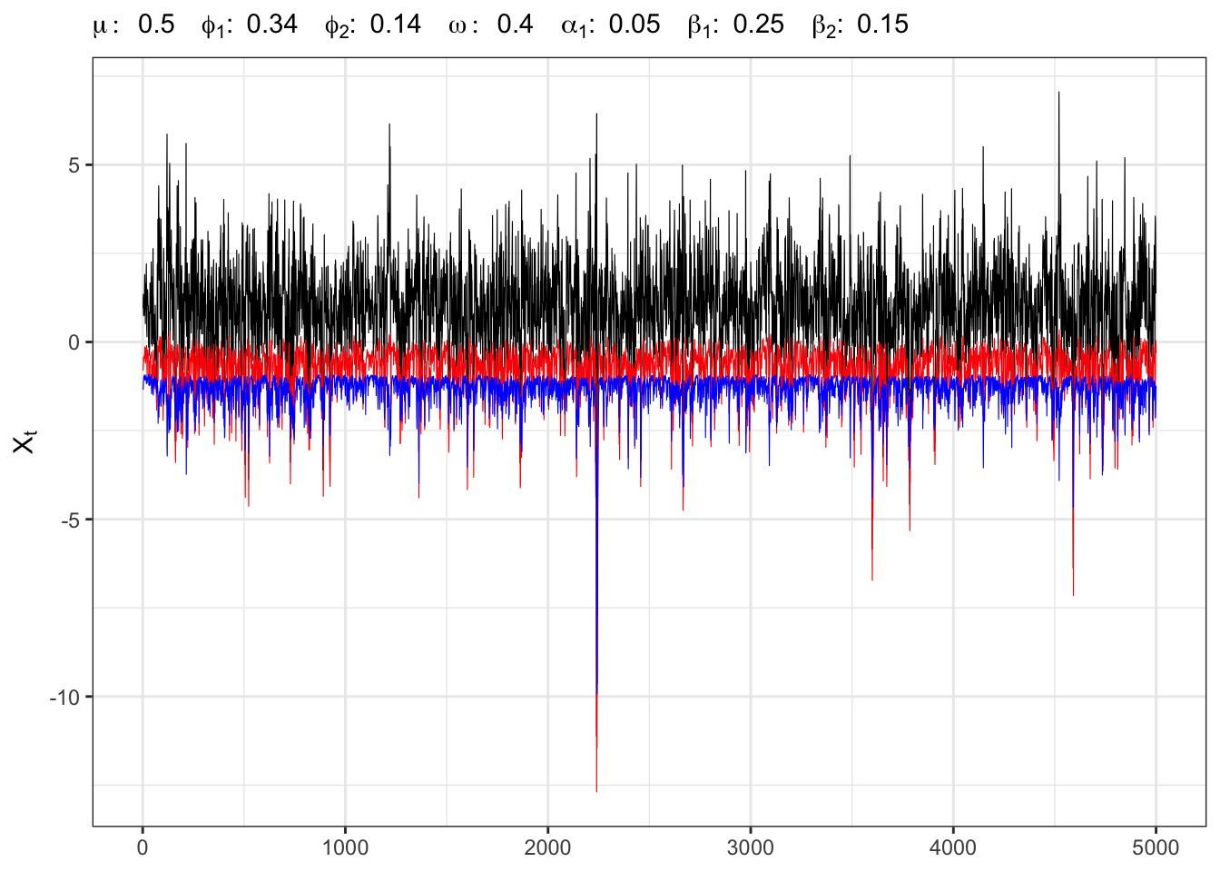
Finally, let’s perform a test on the number of violations.
VaR test
# Violation of the VaR
Vt <- ifelse(Xt < VaR_alpha, 1, 0)
Vt[1:3] <- 0
# Theoretical variance
v_theoric <- alpha*(1-alpha)
# Empirical variance
v_empiric <- (sum(Vt)/t_bar)*(1 - sum(Vt)/t_bar)
# Standardized number of violations
Sn <- sum((Vt - alpha)/sqrt(v_theoric))
# Statistic test (NV_1)
T1 <- (1/sqrt(t_bar)) * Sn
# Statistic test (NV_2)
T2 <- sqrt(v_theoric/v_empiric) * T1
# Rejection level
t_alpha <- qnorm(alpha / 2)| \[n\] | \[\alpha\] | \[\frac{N_n}{n}\] | \[t_{\alpha/2}\] | \[\text{T}_1^{\alpha}\] | \[\text{T}_2^{\alpha}\] | \[t_{\alpha/2}\] | \[\mathcal{H}_0(\text{T}_1)\] | \[\mathcal{H}_0(\text{T}_2)\] |
|---|---|---|---|---|---|---|---|---|
| 5000 | 5% | 5.08% | -1.96 | 0.2596 | 0.2576 | 1.96 | Non-Rejected | Non-Rejected |
Example 26.3 Let’s consider an AR(2)-GARCH(1,2) process of the form \[ \begin{aligned} & {} Y_t = \mu + \phi_1 Y_{t-1} + \phi_2 Y_{t-2} + e_t \\ & e_t = \sigma_t u_t \\ & \sigma_t^2 = \omega + \alpha_1 e_{t-1}^{2} + \beta_1 \sigma_{t-1}^{2} + \beta_2 \sigma_{t-2}^{2} \end{aligned} \] where \(u_t\) is a standardized Student-t innovation with 5 degrees of freedom, namely a heavy-tailed distribution far from the normal one.
AR(2)-GARCH(1,2) simulation
set.seed(1)   # random seed
# *************************************************
#                      Inputs
# *************************************************
# Number of steps ahead
t_bar <- 5000
# Long-term mean
mu <- 0.5
# AR parameters
phi <- c(phi1 = 0.34, phi2 = 0.14)
# Intercept GARCH
omega <- 0.4
# ARCH parameters
alpha <- c(alpha1=0.25)
# GARCH parameters
beta <- c(beta1=0.25, beta2=0.15)
# *************************************************
#                   Simulation
# *************************************************
# Long term mean GARCH variance
e_sigma2 <- omega / (1 - sum(alpha) - sum(beta))
# Long term mean AR
e_Xt <- mu / (1 - sum(phi))
# Initialization
Xt <- rep(e_Xt, 2)
sigma2_t <- rep(e_sigma2, 2)
mu_t <- rep(e_Xt, 2)
# Simulated standardized residuals
df_t <- 5
u_t <- rt(t_bar, df_t) / sqrt(df_t/(df_t - 2))
# Simulated residuals
eps <- rep(0, t_bar)
eps[1:2] <- sqrt(sigma2_t[1:2]) * u_t[1:2]
for(t in 3:t_bar){
  # ARCH component
  sum_arch <- alpha[1]*eps[t-1]^2
  # GARCH component
  sum_garch <- beta[1]*sigma2_t[t-1] + beta[2]*sigma2_t[t-2]
  # Conditional variance
  sigma2_t[t] <- omega + sum_arch + sum_garch
  # Simulated residuals
  eps[t] <- sqrt(sigma2_t[t]) * u_t[t]
  # Conditional mean
  mu_t[t] <- mu + phi[1]*Xt[t-1] + phi[2]*Xt[t-2]
  # Simulated AR component
  Xt[t] <- mu_t[t] + eps[t]
}
Then, we compute the VaR with \(\alpha = 0.05\) as in Example 26.1 using the quantile \(q_{\alpha}\) of a standard normal instead of the true distribution.
AR(2)-GARCH(1,2) VaR
# *************************************************
#                      Inputs
# *************************************************
# lower-tail probability
alpha <- 0.05
# *************************************************
# Quantile standard normal
q_alpha <- qnorm(alpha)
# Value at risk
VaR_alpha <- mu_t + sqrt(sigma2_t) * q_alpha
# Empirical quantile
q_alpha_emp <- quantile(u_t, probs = alpha)
# Empirical Value at Risk
VaR_emp <- mu_t + sqrt(sigma2_t) * q_alpha_emp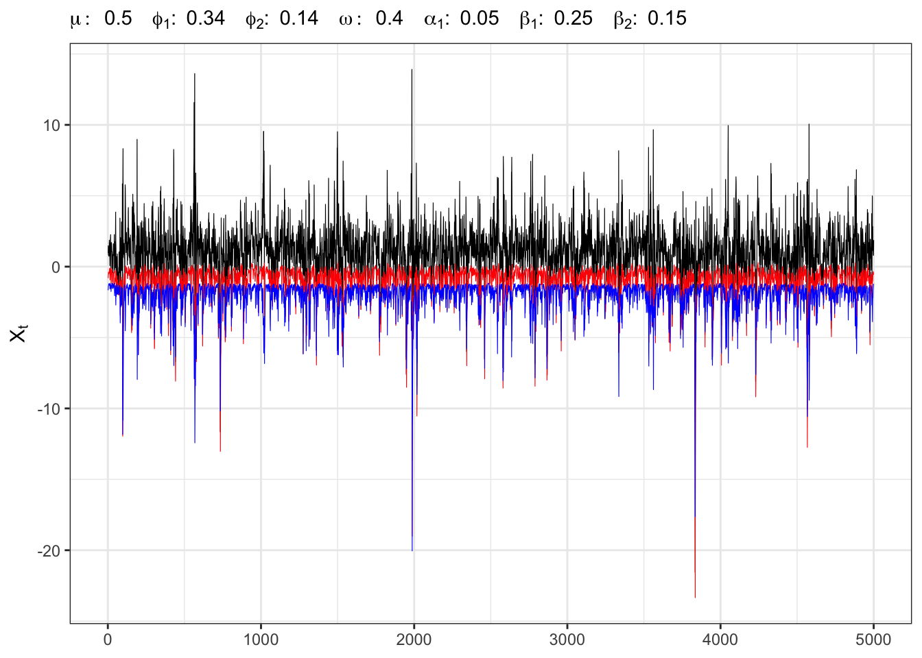
Finally, let’s perform a test on the number of violations.
VaR test
# Violation of the VaR
Vt <- ifelse(Xt < VaR_alpha, 1, 0)
Vt[1:3] <- 0
# Theoretical variance
v_theoric <- alpha*(1-alpha)
# Empirical variance
v_empiric <- (sum(Vt)/t_bar)*(1 - sum(Vt)/t_bar)
# Standardized number of violations
Sn <- sum((Vt - alpha)/sqrt(v_theoric))
# Statistic test (NV_1)
T1 <- (1/sqrt(t_bar)) * Sn
# Statistic test (NV_2)
T2 <- sqrt(v_theoric/v_empiric) * T1
# Rejection level
t_alpha <- qnorm(alpha / 2)| \[n\] | \[\alpha\] | \[\frac{N_n}{n}\] | \[t_{\alpha/2}\] | \[\text{T}_1^{\alpha}\] | \[\text{T}_2^{\alpha}\] | \[t_{\alpha/2}\] | \[\mathcal{H}_0(\text{T}_1)\] | \[\mathcal{H}_0(\text{T}_2)\] |
|---|---|---|---|---|---|---|---|---|
| 5000 | 5% | 4.5% | -1.96 | -1.622 | -1.705 | 1.96 | Non-Rejected | Non-Rejected |